5.2.10. High Pass Filter

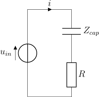
As for the low pass filter we design a high pass filter using just one passive element, in this case a capacitor in series with the driver. In the schemematic below the speaker driver is represented with the resistor.

The transfer function in this case is:

\[H(\omega) = \frac{R}{R+\frac{1}{j\omega C}} = \frac{j\omega RC}{1+j\omega RC}\]

The bode plot for this system with \(R=8\Omega\) and \(C=10\mu F\) is given below. The cutoff frequency appears to be near 2 KHz.

Show code for figure

import numpy as np
import matplotlib.pyplot as plt

plt.clf()

R = 8
C = 10E-6

w = np.logspace(-1,6,num=1000)
H = R / (R+1/(1j*w*C))

plt.plot(w, abs(H))
plt.xscale('log')
plt.yscale('log')
plt.xlabel(r'$\omega$')
plt.ylabel(r'$|H(\omega)|$')
plt.savefig('source/figures/bodeabsplothighpass.png')

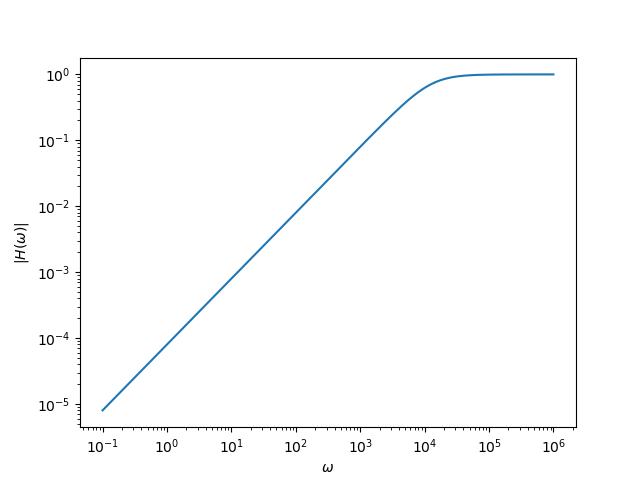
Fig. 5.17 Bode plot of high pass filter.

Let’s do some quick and dirty analysis to see where the cutoff frequency is in terms of R and C. For low frequencies we have

\[H(\omega) \approx j\omega R C\]

and thus

\[\log | H(\omega)| = \log(RC) + \log(\omega)\]

and for large frequencies:

\[H(\omega) \approx 1\]

and thus

\[\log | H(\omega)| = 0\]

The cutoff frequency is thus at \(\omega_x = 1/(RC)\) and for this choice of resistor and capacitor \(f_x = \omega_x/(2\pi) = 1989 Hz\)