5.4.2. From Analog to Digital through the Bilinear Transform
Given a filter designed and specified in the s-domain as a rational function \(H(s)\), there are many ways to turn this filter specification into a discrete filter. The goal for this section is to start with transfer function in the s-domain specifying an analog filter:
and transform it into a discrete filter specified with its transfer function in the z-domain:
Evidently the transform we are looking for needs to know the sample time \(T_s\) to relate the time in the s-domain representation with the samples in the z-domain.
Note that the \(a_n, b_m\) coefficients are certainly not equal to the \(A_n, B_m\) coefficients.
We briefly discuss two of these methods and will discuss a the third method in more detail. The three methods are:
From \(H(s)\) generate the impulse response \(h(t)\) and sample the impulse response to give \(h[n]=h(nT_s)\) where \(T_s\) is the sample time. This method is called the impulse invariance method and works well in case \(H(s)\) represents a FIR filter. But for a true rational filter \(H(s)\) we would rather have a rational function for \(H(z)\) as well to allow for an IIR filter implementation.
A filter specified in the s-domain is completely characterized by its poles and zeros and a gain factor. The same is true for a filter specified in the z-domain. So it seems logical to transform the poles and zeros from the s-domain to poles and zeros in the z-domain. It should be evident that poles/zeros in the s-domain can not be the same as the poles and zeros in the z-domain. Instead the matched Z-transform method uses:
\[z = e^{sT_s}\]where \(s\) is a zero or pole in the s-domain and \(z\) the corresponding zero or pole and \(T_s\) is the sampling time. So in case:
\[H(s) = k_s \frac{\prod_{i=1}^M (s-q_i)}{ \prod_{i=1}^N (s-p_i)}\]we set
\[H(z) = k_z \frac{\prod_{i=1}^M (1-e^{q_i T_s} z^{-1})}{ \prod_{i=1}^N (1-e^{p_i T_s} z^{-1})}\]While it seems like an elegant way to discretize an analog filter it is not often used as it suffers from several disadvantages
neither the time domain impulse response is preserved
nor the frequency domain response.
The most often used discretization method is the bilinear transform method. The starting point for this method is to discretize the s-‘operator’. Remember that a system with transfer function \(s\) differentiates the input signal. So in this method we are looking for an operator in the \(z\)-domain that differentiates the input signal.
5.4.2.1. The Bilinear Transform
We are looking for the discrete time operator that will replace the differentiation operator \(s\) in the continuous time domain.
Forward Difference
A simple approximation is the forward difference operator defined with the relation
where \(T_s\) is the sampling time and \(x[n] = x(nT_s)\). In the z-domain this leads to transfer function \(H(z) = (z-1)/T_s\). Let’s apply the transformation
on the canonical low pass filter
This leads to
For a cut off frequency of \(\w_c = 3 \pi f_c\) for \(f_c=2000 Hz\) and a sample time \(T_s = 1/44100 s\) we plot the frequency response for the continuous time filter and for the discrete time filter.
Show code for figure
 1import numpy as np
 2import matplotlib.pyplot as plt
 3import scipy.signal as sg
 4
 5plt.close('all')
 6
 7fs = 44100
 8Ts = 1/fs
 9fc = 2000
10wc = 2*np.pi*fc
11
12f = np.logspace(1, 5, 1000)
13w = 2 * np.pi * f
14
15Hs = sg.lti([1], [1/wc, 1])
16ws, hs = sg.freqs(Hs.num, Hs.den, worN=w)
17plt.plot(f, 20*np.log10(np.abs(hs)), label='CT filter')
18plt.xscale('log')
19
20
21Hz = sg.dlti([wc*Ts], [1, -1+wc*Ts])
22wz, hz = sg.freqz(Hz.num, Hz.den)
23plt.plot(wz/np.pi*fs/2, 20*np.log10(np.abs(hz)),
24         label=f'Discrete time filter (forward difference)')
25plt.ylim([-20,5])
26
27# Hz = sg.dlti(*sg.bilinear(Hs.num, Hs.den, fs=fs))
28# wz, hz = sg.freqz(Hz.num, Hz.den)
29# plt.plot(wz/np.pi*fs/2, 20*np.log10(np.abs(hz)),
30#          label=f'Discrete time filter (bilinear)')
31# plt.ylim([-20,5])
32
33
34plt.legend()
35
36plt.savefig('source/figures/forward_diff_s2z.png')
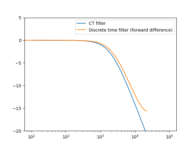
Fig. 5.43 Continuous time low pass filter transformed into a discrete time filter. The frequency response of the canonical first order low pass analog filter is compared with the response of the discrete time filter that is obtained by using a forward difference approximation of the differentiation operator.
The figure above shows that the discretized filter performs according to our expectation. Nevertheless this discretization is method is not without problems. For the continuous time filter the pole is at \(s=-\w_c\), so the analog filter is stable. For the discrete time filter we have a pole at \(z=1-\w_c T_s = 1 - 2\pi f_c/f_s\). Note that the pole is dependent on both the value of the cut off frequency as well as the sampling frequency. For infinitely large \(f_s\) the pole is at \(z=1\) and for lower sampling frequencies the pole moves to the left over the real axis. We van even move it out of the unit circle where the system becomes unstable. So even a system that is stable in the s-domain, this transform based on the forward difference can turn the system into an unstable system in the z-domain.
Bilinear Transform
The bilinear transform is based with a central difference scheme for the estimation of the derivative. Consider the difference equation
The left hand side is an approximation of \(y((n+\frac{1}{2})T_s)\) and the right hand side is an approximation of \(x'((n+\frac{1}{2})T_s)\). The Z-transform of the system that is characterized by the above difference equation is easily calculated and leads to the bilinear transform:
Show code for figure
 1import numpy as np
 2import matplotlib.pyplot as plt
 3import scipy.signal as sg
 4
 5plt.close('all')
 6
 7fs = 44100
 8Ts = 1/fs
 9fc = 3000
10wc = 2*np.pi*fc
11
12f = np.logspace(0, 5, 1000)
13w = 2 * np.pi * f
14
15Hs = sg.lti([1], [1/wc, 1])
16ws, hs = sg.freqs(Hs.num, Hs.den, worN=w)
17plt.plot(f, 20*np.log10(np.abs(hs)), label='CT filter')
18plt.xscale('log')
19
20
21Hz = sg.dlti([wc*Ts], [1, -1+wc*Ts])
22wz, hz = sg.freqz(Hz.num, Hz.den)
23plt.plot(wz/np.pi*fs/2, 20*np.log10(np.abs(hz)),
24         label=f'Discrete time filter (forward difference)')
25plt.ylim([-20,5])
26
27Hz = sg.dlti(*sg.bilinear(Hs.num, Hs.den, fs=fs))
28wz, hz = sg.freqz(Hz.num, Hz.den)
29plt.plot(wz/np.pi*fs/2, 20*np.log10(np.abs(hz)),
30         label=f'Discrete time filter (bilinear)')
31plt.ylim([-20,5])
32
33plt.axvline(fc)
34plt.axhline(-3)
35
36plt.legend()
37
38plt.savefig('source/figures/bilinear_s2z.png')
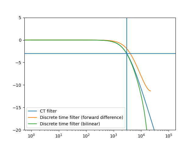
Fig. 5.44 Continuous time low pass filter transformed into a discrete time filter. The frequency response of the canonical first order low pass analog filter is compared with the response of the discrete time filter that is obtained by using a bilinear transform, i.e. a central difference approximation of the differentiation operator.
From the figure we see that the bilinear transformed filter more closely follows the analog filter. Other important observations are
The bilinear transformation maps the entire left half of the s-plane onto the inside of the unit circle in the z-plane, therefore
any stable analog filter with poles on the left side of the imaginary axis will be transformed into a filter with all poles in the unit circle in the z-domain.
The imaginary axis in the s-domain is mapped onto the unit circle, i.e. the frequency transfer function \(H(s)\Bigr|{s=j\w}\) is mapped onto the frequency transfer function \(H(z)\Bigr|{z=e^j\W}\).
The bilinear transformation maps a rational function (a fraction of polynomials) in the s-domain onto a rational function in the z-domain. This guarantees that the resulting digital filter can be efficiently implemented as an IIR filter.
The first two properties guarantee that applying the bilinear transform to a stable filter prototype in the s-domain will result in a stable filter in the z-domain. The third property should be considered with some care. It is evidently impossible to have \(\W = \w\) as \(\w\in\setR\) whereas \(\W\in[-\pi,\pi]\).
The bilinear transform is invertible, we have
So for points \(s=j\w\) on the imaginary axis we have:
where \(|z|=1\) and
Let \(\w = 2\pi f\) where \(f\) is the frequency in Hz in the analog domain. The corresponding frequency in the digital domain \(f_d\) after the bilinear transform then is (see the chapter on the Discrete Time Fourier Transform):
resulting in:
Show code for figure
 1import numpy as np
 2import matplotlib.pyplot as plt
 3import scipy.signal as sg
 4
 5plt.close('all')
 6
 7fs = 44100
 8f = np.linspace(-fs, fs, 1000)
 9fd = fs / np.pi * np.arctan(np.pi * f / fs)
10plt.plot(f, fd)
11plt.plot(f, f)
12plt.xlabel(f'Analog frequency $f$')
13plt.ylabel(f'Digital frequency $f_d$')
14plt.savefig('source/figures/freqwarp_s2z.png')
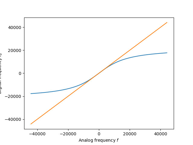
Fig. 5.45 Frequency warping by the bilinear transform. For sample frequency \(f_s=44100\) the warped digital frequency \(f_d\) is plotted. Note that for lower frequencies the warping is quite accurate but for larger frequencies deviates from the original frequency.
5.4.2.2. Pre-Warping
To correct for the frequency warping often a pre-warping is used. Consider a second order analog filter \(H(s)\) characterized with a natural frequency \(\w_0\). In order to map the natural frequency to the correct frequency after the bilinear transform we select an analog frequency \(\w'_0\) such that after the bilinear transform this frequency is mapped to the correct value \(\w_0\). For this we use the warping expression for the radial frequency:
leading to:
Rearranging terms and taking the \(\tan\) on both sides of the equation leads total
i.e.