1.2.4. Basic Signals¶

The basic signals we will discuss in this section are seldomly encountered in real life. Nevertheless they are essential in signal processing as they are the building blocks in decomposing a signal into the basic signals (especcially the complex exponential function) and characterizing systems by looking at their response to these basic signals.

1.2.4.1. Constant Signal¶

The constant signal (function) is easy:

	CT	DT
Constant Function	$x(t) = 1$	$x[n] = 1$

and we can use any constant instead of 1 (even complex valued constants).

1.2.4.2. Step Function¶

A step function is far more important and far more common then you might think. When you hit the light switch at time $t=0$ and you think of the lamp as a system that is fed the electrical signal $x(t)$ as input and outputs light (with measured intensity $y(t)$), this system is fed with a step function. For $t<0$ there was no voltage difference at the lamp and then suddenly from time $t=0$ and onwards the lamp is fed with a 230 V electrical signal.

What happens in the lamp system? When there is voltage applied to the lamp (we think of an old fashioned lamp) current starts to flow through the filament (a piece of wire) and the filament starts to heat up (filaments have the property to give a lot a light when heated). After a (short) while there is an equilibrium, the filament is at a constant temperature and thus the output $y(t)$ is constant. But what happens between time $t=0$ and the time the equilibrium settles in?

Yes the above explanation of a lamp turned on does fit into these lecture series. The transition the lamp makes from off to on is called the step response of the system. When we are looking at control theory at the end of these lectures series we will look into this at more detail.

	CT	DT
Step Function	$x(t) = \begin{cases} 0 &: t<0\\ 1 &: t\geq 0\end{cases}$	$x[n] = \begin{cases} 0 &: n<0\\ 1 &: n\geq 0\end{cases}$

1.2.4.3. Pulse Function¶

The pulse function, also called the impulse function, in DT is easy: everywhere zero except at $n=0$ where the values is $1$. The DT pulse is written as $\delta[n]$.

In CT it is more difficult. The pulse in CT is written as $\delta(t)$. It is mathematically defined with the sifting property:

\[x(0) = \int_{-\infty}^{\infty} x(t)\delta(t)dt\]

Don’t worry in case you cannot make much sense out of this property. It is not even an (Stieltjes) integral that we are used to.

A usefull way to think about a pulse signal is to consider a signal in which you want to concentrate a finite amount of energy in a short a time interval as possible. Energy in a signal is measured by integrating a signal over a period of time.

Consider for instance the signal $x_a(t)$ defined as:

(1.1)¶\[\begin{split}x_a(t) = \begin{cases} \frac{1}{2a} &: -a \leq t \leq a\\ 0 &: \text{elsewhere} \end{cases}\end{split}\]

The total energy in this signal (1.1) is $1$ (the integral of $x(t)$ over the entire domain). This is true irrespective of the value of $a$. In the limit when $a\rightarrow0$ the value $x_a(0)\rightarrow\infty$ but still the total area under the function remains 1. In a sloppy way we may define:

\[\delta(t) = \lim_{a\rightarrow0} x_a(t)\]

The strange thing thus is that the function value is infinite (well more accurate said it is not well defined) at $t=0$ whereas the integral over the entire domain is finite and equal to 1.

We will see many uses of the pulse function. The translated and scaled CT pulse function $3 \delta(t-2)$ is plotted as:

Show code for figure

import numpy as np
import matplotlib.pyplot as plt

plt.clf()
n = np.arange(10);
x = np.zeros_like(n);
plt.stem([2], [3], markerfmt='^b', linefmt='blue', use_line_collection=True);
plt.plot(n, x, 'b')
plt.savefig('source/figures/pulseplot.png')

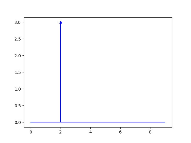
Fig. 1.9 Shifted Pulse function $\delta(t-2)$.¶

The straight line indicates it is a pulse and the length of the line indicates the total energy. To distinguish a continuous pulse function from a discrete time funtion we mark the stem (the vertical line) with an upward arrow.

We can sum several pulse functions (which we will often do later on in the course), e.g.:

\[x(t) = 3\delta(t-2) + 2\delta(t-3)\]

This looks like:

Show code for figure

plt.clf()
n = np.arange(10);
x = np.zeros_like(n);
plt.stem([2,3], [3,2], markerfmt='^b', linefmt='blue', use_line_collection=True);
plt.plot(n, x, 'b')
plt.savefig('source/figures/twopulseplot.png')

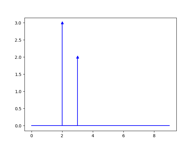
Fig. 1.10 Added Pulse functions $3\delta(t-2)+2\delta(x-3)$.¶

Summarizing we have:

	CT	DT
Definition	$x(t) = \delta(t) \equiv \lim_{a\rightarrow0} x_a(t)$	$x[n] = \delta[n] \equiv \begin{cases} 1 &: n=0\\ 0 &: \text{elsewhere} \end{cases}$
Sieve Property	$\int_{-\infty}^{\infty} x(t)\delta(t-a)dt = x(a)$	$\sum_{n=-\infty}^{\infty} x[n]\delta[n-a] = x[a]$

We leave the proofs for the sieve properties to the reader. These properties are needed in subsequent sections of these notes.

1.2.4.4. Complex Exponential Functions¶

Continous Time

The CT complex exponential function is

\[x(t) = e^{j\w t} = \cos(\w t) + j\sin(\w t)\]

Easy to prove properties of this function are:

Periodicity. The CT complex exponential function is periodic with period $2\pi/\w$.
Magnitude. The magnitude is $|e^{j\w t}| = 1$.
Angle. The angle or phase is $\angle e^{j\w t} = \w t$ is expressed in radians. The angular velocity (hoeksnelheid) is expressed in radians per second.

In the section on plotting complex signals the function $\exp(100\pi t)$ is plotted in the classical two ways (imaginary and real part as function of time, and magnitude and angle as function of time).

For a complex exponential it is sometimes useful to depict the function as a path in the complex plane. If we start at $t=0$ we are in the point $1+0j$ then increasing $t$ we follow a circular path around the origin. For $t=2\pi/w$ we return in the origin after following the entire unit circle once. The ‘speed’ along the path is determined by the angular velocity $\w$.

Discrete Time

The DT exponential signal is:

\[x[n] = e^{j\Omega n} = \cos(\Omega n) + j\sin(\Omega n)\]

For this discrete function to be periodic we must have:

\[\begin{split}x[n+T] = x[n]\\ e^{j\Omega (n+T)} = e^{j\Omega n}\\ e^{j\Omega T}e^{j\Omega n} = e^{j\Omega n}\end{split}\]

i.e.

\[e^{j\Omega T} = 1\]

and thus

\[\Omega T = k 2\pi\quad\forall k\in\setZ\]

or

\[T = \frac{k 2 \pi}{\Omega}\]

Please note that $T$ should be an integer and that is certainly not guaranteed for all $\Omega$. It is only guaranteed in case $\Omega/\pi$ is a rational number.

The properties of the DT complex exponential function are:

Periodicity. The discrete exponential signal is periodic only in case $\Omega/\pi$ is a rational number.
Magnitude. The magnitude is $|e^{j\Omega n}| = 1$
Angle. The angle or phase is $\angle e^{j\Omega n} = \Omega n$. Note that the $\Omega$ is expressed in radians as opposed to $\omega$ that is expressed in radians per second.

Summarizing:

Table 1.1 **Complex Exponential Function**¶
	CT	DT
Definition	$x(t) = e^{j\w t}$	$x[n] = e^{j\Omega n}$
Periodicity	periodic with $T=2\pi/\omega$	periodic in case $\Omega/\pi$ is rational$

1.2.4.5. Chirp Signal¶

The chirp or sweep signal is a semi periodic signal. Think of an audio signal that increases its frequency starting at time $t_0=0$ at frequency $f_0$ and after $t_1$ seconds ends at frequency $f_1$.

A sweep signal is very useful in practice to test a system at a lot of frequencies.

We start with a cosine function, but instead of defining $\cos(2\pi f t)$ we define:

\[x(t) = \cos(\Phi(t))\]

where $\Phi$ is the angle or phase function. The instantaneous frequency can then be found with

\[\cos(\Phi(t+T)) = \cos(\Phi(t)+2\pi)\]

or:

\[\Phi(t+T) = \Phi(t)+2\pi\]

Note that $T$ is a function of $t$. In first order approximation we can write:

\[\Phi(t) + T(t)\Phi'(t) = \Phi(t)+2\pi\]

or:

\[T(t)\Phi'(t) = 2\pi, \qquad \frac{d\Phi(t)}{d t} = \frac{2\pi}{T(t)} = \w(t) = 2\pi f(t)\]

where $\w(t)$ is the instantaneous radial frequency and $f(t)$ is the instantaneous frequency in Hz. For a linear sweep we would like the frequency to start at $f_0$ and with time linearly increase to $f_1$ at time $t_1$”:

\[f(t) = f_0 + \frac{f_1-f_0}{t_1} t\]

So

\[\frac{d\Phi(t)}{d t} = 2\pi\left( f_0 + \frac{f_1-f_0}{t_1} t \right)\]

and thus:

\[\Phi(t) = 2\pi\left( f_0 t + \frac{f_1-f_0}{2 t_1} t^2 \right) + \Phi_0\]

Thus a sweep or chirp is generated with:

\[x(t) = \cos\left( 2\pi\left( f_0 t + \frac{f_1-f_0}{2 t_1} t^2 \right) + \Phi_0\right)\]

Show code for figure

plt.clf()
f0 = 1
f1 = 5
t1 = 5
t = np.linspace(0, t1, 1000);
x = np.cos(2*np.pi*(f0*t + (f1-f0)/2/t1 * t**2))
plt.plot(t, x);
plt.xlabel('t');
plt.ylabel('x(t)');
plt.title('Chirp Signal');
plt.savefig('source/figures/chirp.png')

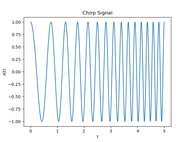
Fig. 1.11 Linear Chirp Signal.¶

In the code below an audio chirp signal is generated and written to a wav file. This file can be played in any modern browser. The chirp starts at 100 Hz and over a period of 5 seconds ends at 10000 Hz. Maybe younger ears do better but the higher frequencies for me are noticeably attenuated (and 10 kHz is only halfway up to the maximum frequency of 20 kHz that the human ear can perceive).

f0 = 100
f1 = 10000
t1 = 5
t = np.linspace(0, t1, t1*44100);
x = np.cos(2*np.pi*(f0*t + (f1-f0)/2/t1 * t**2))

import scipy.io.wavfile as wf
wf.write('source/_static/chirp.wav', 44100, np.int16(np.iinfo(np.int16).max * x))