3.2. Continuous Time Fourier Transform

3.2.1. The Fourier Transform

Now we consider functions \(x(t)\) that are not (necessarily) periodic. In this case there are not necessarily such things as a fundamental period and a fundamental frequency. Therefore to synthesize a signal \(x(t)\) we need all frequencies.

\[x(t) = \frac{1}{2\pi} \int_{-\infty}^{\infty} X(\w)e^{j\w t}d\omega\]

We see that \(X(\w)\) determines the weight (relative importance) of the exponential function \(\exp(j\w t)\) in the synthesis of the signal \(x(t)\). That function \(X(\w)\) is called the Fourier transform of \(x(t)\) and will denoted by \(X(\w) = \FT(x(t))\)

We will often write:

\[x(t) \xrightarrow{\quad\FT\quad} X(\w)\]

The Fourier transform (the analysis equation) is given by

\[X(\w) = \int_{-\infty}^{\infty} x(t) e^{-j\w t} dt\]

As there is a one to one correspondence between a signal and its Fourier transform we can also write:

\[x(t) \xleftarrow{\quad\IFT\quad} X(\w)\quad\text{or}\quad X(\w) \xrightarrow{\quad\IFT\quad} x(t)\]

This arrow diagram evidently refers to the inverse Fourier transform \(\IFT\) or the synthesis equation.

3.2.2. Properties of the CT Fourier Transform

First we present some of the properties of the Fourier transform. In later sections we will provide some proofs and some uses and consequences of these properties.

Time Domain	Frequency Domain
Synthesis (Inverse Fourier Transform) \[x(t) = \frac{1}{2\pi} \int_{-\infty}^{\infty} X(\w)e^{j\w t}d\omega\]	Analysis (Fourier Transform) \[X(\w) = \int_{-\infty}^{\infty} x(t) e^{-j\w t} dt\]
Real Signals \[x(t) \in\setR\]	Symmetry in Fourier transform \[X(-\w) = X^\star(\w)\]
Even Signals \[x(-t) = x(t)\]	Real Fourier transform \[X(\w) \text{ is real and even}\]
Odd Signals \[x(-t) = -x(t)\]	Imaginary Fourier transform \[X(\w) \text{ is imaginary and odd}\]
Derivative \[x'(t) = \frac{d}{dt} x(t)\]	High frequency gain \[j\w X(\w)\]
Time scaling \[x(a t)\]	Frequency scaling \[\frac{1}{|a|}X(\frac{\w}{a})\]
Convolution \[x(t) \ast y(t) = \int_{-\infty}^{\infty} x(t-u) y(u) du\]	Multiplication \[X(\w) Y(\w)\]
Multiplication \[x(t) y(t)\]	Convolution \[\frac{1}{2\pi} X(\w) \ast Y(\w)\]
Duality \[\begin{split}x(t)\\ X(t)\end{split}\]	\(\hspace{1em}\) \[\begin{split}X(\w)\\ 2\pi x(-\w)\end{split}\]

3.2.2.1. Real Signals

Let \(x(t)\) be a real valued signal. For the Fourier transform \(X(\w)\) we can write:

\[\begin{split}X(\w) &= \int_{-\infty}^{\infty} x(t)\left(\cos(\w t)- j \sin(\w t)\right)dt\\ &= \int_{-\infty}^{\infty} x(t)\cos(\w t)dt - j\int_{-\infty}^{\infty} x(t)\sin(\w t)dt\end{split}\]

For \(X(-\w)\) we get

\[\begin{split}X(-\w) &= \int_{-\infty}^{\infty} x(t)\left(\cos(\w t) + j \sin(\w t)\right)dt\\ &= \int_{-\infty}^{\infty} x(t)\cos(\w t)dt + j\int_{-\infty}^{\infty} x(t)\sin(\w t)dt\end{split}\]

Showing that \(X(-\w) = X^\star(\w)\). The consequence of this symmetry in the Fourier transform is that when plotting the Fourier transform we only have to consider the positive frequencies.

3.2.2.2. Even and Odd Signals

We start by rewriting the definition of the Fourier transform:

\[\begin{split}X(\w) &= \int_{-\infty}^{\infty} x(t)e^{-j\w t}dt\\ &= \int_{-\infty}^{0} x(t)e^{-j\w t}dt + \int_{0}^{\infty} x(t)e^{-j\w t}dt\\ &= \int_{0}^{\infty} x(-t)e^{j\w t}dt + \int_{0}^{\infty} x(t)e^{-j\w t}dt\end{split}\]

For an even signal we have \(x(-t)=x(t)\) and thus

\[\begin{split}X(\w) &= \int_{0}^{\infty} x(t)e^{j\w t}dt + \int_{0}^{\infty} x(t)e^{-j\w t}dt\\ &= \int_{0}^{\infty} x(t)\left( e^{j\w t}+e^{-jwt} \right)\\ &= 2 \int_{0}^{\infty} x(t)\cos(\w t) dt\end{split}\]

For a real and even signal we see that the Fourier transform is real valued. Furthermore \(X(\w)\) is an even function (note that the product of two even functions (\(x(t)\) and \(\cos(\w t)\) is even too).

Along the same line of reasoning it can be shown that the Fourier transform of an odd signal is purely imaginairy and odd.

3.2.2.3. Derivatives

Let

\[x(t) \FTright X(\w)\]

then:

\[x'(t) \FTright j\w X(\w)\]

The proof simply follows from the synthesis equation:

\[x(t) = \frac{1}{2\pi} \int_{-\infty}^{\infty} X(\w) e^{j\w t}dw\]

Differentiating with respect to \(t\) on both sides of the equation and using Leibnitz integration rule we get

\[\begin{split}x'(t) &= \frac{1}{2\pi} \int_{-\infty}^{\infty} X(\w) \frac{d}{dt}e^{j\w t}dw\\ &= \frac{1}{2\pi} \int_{-\infty}^{\infty} X(\w) j\w e^{j\w t}dw\end{split}\]

From this equation we see that \(j \w X(\w)\) is the Fourier transform of \(x'(t)\).

3.2.2.4. Pulse Function

Let \(x(t)=\delta(t)\), this pulse function ‘contains’ all frequencies in a equal amount, i.e. \(X(\w)=1\). This is evidently true given the sieve property of a pulse function.

\[\delta(t) \FTright 1\]

For a shifted pulse we have

\[\delta(t-t_0) \FTright e^{-j\w t_0}\]

3.2.2.5. Time Shifts

The Fourier transform of a shifted function \(y(t) = x(t-t_0)\) is:

\[\begin{split}Y(\w) &= \int_{-\infty}^{\infty} y(t)e^{-j\w t} dt\\ &= \int_{-\infty}^{\infty} x(t-t_0) e^{-j\w t} dt\end{split}\]

changing to variable \(t' = t - t_0\) we get:

\[\begin{split}Y(\w) &= \int_{-\infty}^{\infty} x(t') e^{-j\w (t'+t_0)} dt'\\ &= e^{-j\w t_0} \int_{-\infty}^{\infty} x(t') e^{-j\w t'} dt'\\ &= e^{-j\w t_0} X(\w)\end{split}\]

So

\[x(t-t_0) \FTright e^{-j\w t_0} X(\w)\]

3.2.2.6. Complex Exponential

A complex exponential function \(x(t)=e^{j\w_0 t}\) contains just one frequency \(\w_0\) so its Fourier transform be a pulse at that frequency. And indeed we can prove:

\[e^{j\w_0 t} \FTright 2\pi \delta(w-\w_0)\]

If you start in the time domain and use the Fourier transform you end up with the need to prove that:

\[\int_{-\infty}^{\infty} e^{j (w-w_0) t} dt\]

is a pulse at \(w_0\). It is simpler in this case to start with the pulse in the frequency domain and calculate its inverse Fourier transform:

\[\frac{1}{2\pi} \int_{-\infty}^{\infty} 2\pi \delta(\w - \w_0) e^{j\w t} d\w = e^{j\w_0 t}\]

3.2.2.7. Periodic Signal

Let \(x(t)\) be a periodic signal, i.e. \(x(t+T_0)=x(t)\) then we calculate the Fourier Series coefficients \(a_k\) and write:

\[x(t) = \sum_{k=-\infty}^{\infty} a_k e^{j k \w_0 t}\]

where \(\w_0 = 2\pi/T_0\). This expression for \(x(t)\) can be used to calculate the Fourier transform (not the series coefficients) of \(x(t)\):

\[\begin{split}X(\w) &= \int_{-\infty}^{\infty} x(t) e^{-j\w t} dt\\ &= \int_{-\infty}^{\infty} \left( \sum_{k=-\infty}^{\infty} a_k e^{j k \w_0 t} \right) e^{-j\w t} dt\\\end{split}\]

Interchanging sum and integration

\[X(\w) = \sum_{k=-\infty}^{\infty} a_k \int_{-\infty}^{\infty} e^{j k \w_0 t} e^{-j\w t} dt\]

where the integral is the Fourier transform of \(e^{jk\w_0 t}\) which was shown to be \(2\pi \delta(\w-k\w_0)\) and so:

\[X(\w) = 2\pi \sum_{k=-\infty}^{\infty} a_k \delta(\w-k\w_0)\]

showing that the Fourier transform of a periodic function is a modulated pulse train. The energy in the pulse at \(\w=k \w_0\) is equal to \(2\pi a_k\).

3.2.2.8. Pulse Train

Consider the pulse train

\[x(t) = \sum_{k=-\infty}^{\infty} \delta(t - kT_0)\]

Somewhat suprisingly its Fourier transform is a pulse train as well:

\[X(\w) = \w_0 \sum_{k=-\infty}^{\infty} \delta(\w-k\w_0)\]

The proof is easy when you realize that the pulse train is a periodic function with period \(T_0\). For this periodic function we can calculate the Fourier coefficients \(a_k\):

\[\begin{split}a_k &= \frac{1}{T_0} \int_{-T_0/2}^{T_0/2} \delta(t) e^{-j k\w_0 t}dt\\ &= \frac{1}{T_0}\end{split}\]

(remember the sieve property of the delta function?). Now we can use the result for any periodic function and substitute the \(a_k\) for the pulse train:

\[\begin{split}X(\w) &= 2\pi \sum_{k=-\infty}^{\infty} a_k \delta(\w-k\w_0)\\ &= \frac{2\pi}{T_0} \sum_{k=-\infty}^{\infty} \delta(\w-k\w_0)\\ &= \w_0 \sum_{k=-\infty}^{\infty} \delta(\w-k\w_0)\end{split}\]

3.2.2.9. Convolution

Given two signal \(x(t)\) and \(y(t)\) with Fourier transforms \(X(\w)\) and \(Y(\w)\) respectively. Then

\[\begin{split}x(t) \ast y(t) &\FTright X(\w)Y(\w)\\ x(t)y(t) &\FTright \frac{1}{2\pi} X(\w) \ast Y(\w)\end{split}\]

3.2.2.10. Duality

The duality principle for Fourier analysis states that if we have a Fourier transform pairs

\[x(t) \FTright X(\w)\]

we also have:

\[X(t) \FTright 2\pi x(-\w)\]

3.2.3. Fourier Transform Pairs

First we present some basic and often needed Fourier transform pairs. Proofs of some of these pairs will be given later on.

Time Domain	Frequency Domain
Synthesis \[x(t) = \frac{1}{2\pi} \int_{-\infty}^{\infty} X(\w)e^{j\w t}d\omega\]	Analysis \[X(\w) = \int_{-\infty}^{\infty} x(t) e^{-j\w t} dt\]
Pulse \[x(t) = \delta(t)\]	Constant \[X(\w) = 1\]
Finite Pulse \[\begin{split}x(t) = \begin{cases} 1/2 &: -1 \leq x \leq 1\\ 0 &: \text{elsewhere} \end{cases}\end{split}\]	Sinc \[X(\w) = \frac{\sin(\w)}{\w}\]
Complex Exponential \[e^{j\w_0 t}\]	Pulse \[2\pi \delta(\w-\w_0)\]
Cosine \[\cos(\w_0 t)\]	Pulses \[\pi( \delta(\w-\w_0) + \delta(\w+\w_0) )\]
Sine \[\sin(\w_0 t)\]	Pulses \[\frac{\pi}{j} (\delta(\w-\w_0) - \delta(\w+\w_0) )\]
Pulse train \[\sum_{n=-\infty}^{\infty} \delta(t - nT)\]	Pulse train \[\frac{2\pi}{T} \sum_{k=-\infty}^{\infty} \delta\left( \w - \frac{2\pi k}{T}\right)\]

The proof of some of these pairs will be left as an exercise to the reader in the exercises section. Some will be proven below.

3.2.3.1. Complex Exponential \(\FTright\) Pulse

To prove the Fourier transform pair \(e^{j\w_0 t}\FTright 2\pi\delta(\w - \w_0)\) we could start with the complex exponential and use the Fourier transform definition. That will result in a difficult integral to calculate. It is easier to start with the pulse in the frequency domain and use the inverse Fourier transform:

\[\begin{split}\IFT\{2\pi\delta(\w-\w_0)\} &= \frac{1}{2\pi}\int_{-\infty}^{\infty} 2\pi\delta(\w-\w_0)e^{j\w t}d\w\\ &= \int_{-\infty}^{\infty} \delta(\w-\w_0)e^{j\w t}d\w\\ &= e^{j\w_0 t}\end{split}\]

In the last step we have used the sifting property of the pulse function.

3.2.3.2. Pulse \(\FTright\) Complex Exponential

We can use the duality principle to derive a new transform pair from the one stated just above:

\[e^{j\w_0 t} \FTright 2\pi \delta(\w-\w_0)\]

Applying the duality property we gettext

\[2\pi \delta(t-t_0) \FTright 2\pi e^{-j t_0 \w}\]

or

\[\delta(t-t_0) \FTright e^{-j \w t_0}\]

The correctness can be easily verified by directly calculating the Fourier transform of the shifted pulse or alternatively using the shifting property on the transform pair \(\delta(t)\FTright 1\).

3.2.4. Bode Plots

Consider a continuous time LTI system characterized with impulse response function \(h(t)\) with Fourier transform \(H(\w)\). To assess the way this system processes the individual frequencies a plot of \(|H(\w)|\) and \(\angle H(\w)\) as function of the (radial) frequency \(\w\) is made.

As an example consider a simple system with transfer function

\[H(\w) = \frac{1}{1+j\frac{\w}{\w_c}}\]

It is customary to plot both \(|H(\w)|\) and \(\w\) on a logaritmic scale. For the value (vertical) axis this is done by expressing the magnitude in decibels:

\[20 \log_{10} |H(\w)|\]

Show code for figure

import numpy as np
import matplotlib.pyplot as plt


def bode_plot(w, H, zorder=2, xscale='log',
              title='Bode plot',
              xlabel=r'$\omega$',
              ylabel=r'$H(\omega)$'):
    fig, (axabs, axangle) = plt.subplots(2)

    axabs.plot(w, 20 * np.log10(np.abs(H)), lw=3, zorder=zorder)
    axabs.set_xlabel(xlabel)
    axabs.set_ylabel(r'$|$' + ylabel + r'$|$')
    axabs.set_xscale(xscale)
    axabs.grid(True, which='both')
    axabs.set_title(title)

    axangle.plot(w, np.angle(H), lw=3, zorder=zorder)
    axangle.set_xlabel(xlabel)
    axangle.set_ylabel(r'$\angle$ '+ ylabel)
    axangle.set_xscale(xscale)
    axangle.grid(True, which='both')

    fig.subplots_adjust(wspace=0)

    return fig, (axabs, axangle)


f = np.logspace(1,5)
fc = 2000
def H(w):
    return 1/(1+1j*w)

title=r'Bode plot for $H(\omega)=\frac{1}{1+j \omega/\omega_c}$'
fig, (axabs, axangle) = bode_plot(f, H(f/fc), xscale='log',
                                  title=title,
                                  xlabel=r'frequency $f$', ylabel=r'$H(2\pi f)$')
axabs.axvline(2000)
axangle.axvline(2000)
absHend = 20 * np.log10(np.abs(H(1E5/fc)))
axabs.plot([1E1, fc, 1E5], [0, 0, absHend], lw=7, color='red', alpha=0.4, zorder=1)
plt.savefig('source/figures/lowpassplotloglog.png')

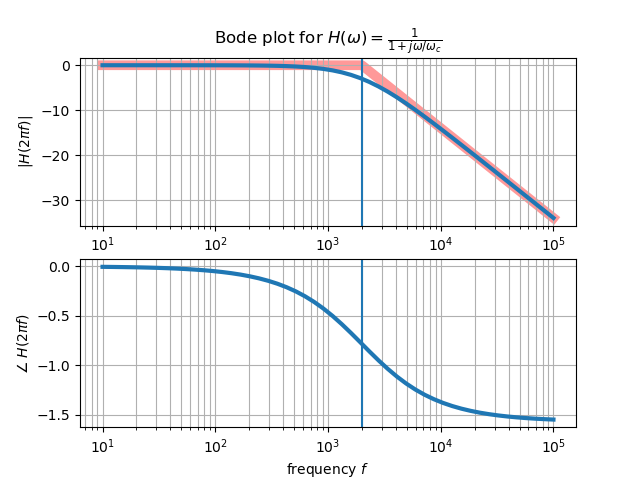
Fig. 3.6 Bode plot for the transfer function \(H(\w) = \frac{1}{1+j \omega/\omega_c}\) where the cut off frequency \(\w_c = 2\pi f_c\) with \(f_c = 2000 \text{Hz}\). In the plot the cut off frequency is indicated with a vertical blue line. The asymptotic behavior of \(|H(\w)|\) is sketched with the faint red lines.

3.2.5. Exercises

1. Odd Signals

   Give a proof that the Fourier transform \(X(\w)\) of a real and odd signal \(x(t)\) is purely imaginairy.

2. Finite Pulse Signal

   Give a proof that the Fourier transfor of the finite pulse function (or block function):

   \[\begin{split}x(t) = \begin{cases} 1/2 &: -1 \leq x \leq 1\\ 0 &: \text{elsewhere} \end{cases}\end{split}\]

   is given by

   \[X(\w) = \frac{\sin\w}{\w}\]

3. Sine and Cosine

   Calculate the Fourier transform of \(\sin(\w t)\) and \(\cos(\w t)\). The anwers are not enough (these are in the table above), you should give a proof.

4. Impulse response

   Calculate the Fourier transform \(H(\w)\) of the function \(h(t)\),

   \[h(t) = e^{-t} u(t)\]

   where \(u(t)\) is the step function.

5. Linear System Response

   The function \(h(t)\) is the impulse response function of a linear system that is known as a low pass filter.

   1. Make a Bode plot of \(H(\w)\) (i.e. on logarithmic scales) and show that frequencies below \(\w=1\) are passed unchanged by this filter whereas frequencies above \(\w=1\) are decreased in amplitude.

   2. Consider the signal:

      \[x(t) = 5 \sin(0.5t) + \sin(2 t)\]

      Plot this signal. You see a low frequency sinusoid of large amplitude with a high frequency small ampliture sinusoid added to it.

   3. Calculate the Fourier transform \(X(\w)\) of \(x(t)\).

   4. The linear system characterized with impulse response \(h(t)\) is fed with input signal \(x(t)\) to produce output signal \(y(t)\). Calculate \(y(t)\). Hint: use the convolution property of the Fourier transform.

      Plot \(x(t)\) and \(y(t)\) in the same figure.

6. Finite Width Impulse \(\FTright\) Sinc

   Consider the finite width pulse function:

   \[\begin{split}x_a(t) = \begin{cases} 1/(2a) &: -a \leq x \leq a\\ 0 &: \text{elsewhere} \end{cases}\end{split}\]

   Calculate the Fourier transform \(X_a(\w)\) and plot both \(x_a(t)\) and \(X_a(\w)\) for \(a=1,2,3\).

7. Convolution

   Give a proof of the convolution property:

   \[x(t)\ast y(t) \FTright X(\w)Y(\w)\]

   The most elegant proof will be presented in the lecture notes for future students.

8. Example

   Consider the real valued, even function \(x(t)\) whose Fourier spectrum \(|X(\w)|\) is

   \[\begin{split}|X(\w)| = \begin{cases} 1 - \frac{\w}{\w_0} &: 0\leq\w<\w_0\\ 0 &: \w \geq \w_0 \end{cases}\end{split}\]

   and is sketched in the figure below (with \(\w_0=2\))

   Show code for figure

   import numpy as np
   import matplotlib.pyplot as plt
   
   plt.clf()
   
   w0 = 2
   w = np.linspace(0, 6, 100)
   X = np.maximum(0, 1-w/w0)
   
   plt.gcf().set_size_inches(5, 3)
   plt.plot(w, X)
   plt.savefig('source/figures/Xexample.png')
   

   

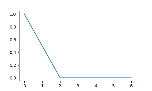
   The Fourier spectrum is only given for the positive \(\w\) values, the rest follows from symmetry principles.

   1. Sketch the spectrum \(|X(\w)|\) for all \(\w\).

   2. What is the Fourier transform \(X(\w)\)? Also give a sketch.

   3. Calculate and plot the signal \(x(t)\). If your integral calculation skills are a bit rusty you can use Mathematica (Wolfram Alpha) or Maple or …

9. Low Pass Filter.

   In a previous subsection we looked at the Bode plot for the system with transfer function

   \[H(\w)=\frac{1}{1+j\frac{\w}{\w_c}}\]

   1. Show that at the cut off frequency \(f_c\) the magnitude of the transfer function is at -3 dB.

   2. Show that for \(f>f_c\) the transfer function magnitude decays with 6 dB per octave (any frequency interval from \(f_0\) to \(2f_0\) is called an octave).

   3. We now make a new filter/system by cascading two systems each with transfer function \(H\). Show that the cascade of two LTI system is an LTI system itself.

   4. Show that the cascade of twp systems each with transfer function \(H\) results in a system with transfer system \(H^2\).

   5. Plot the transfer function \(H^2\) where \(H\) is the function given above.

   6. Calculate the decay for this cascaded system for \(f>f_c\) is 12 dB per octave.