5.3.1. The Sampling Theorem

We are interested in the relation between \(x[n]\) and \(x(t)\) where \(x[n]=x(n T_s)\). However we want our sampled signal to be represented as CT signal as well. In that case we can compare the CT Fourier transform of \(x(t)\) with the Fourier transform of its sampled version and see wether we lost information in the sampling process. In order to do so, we need a mathematical trick that we have used before: we will represent the (sampled) signal as a summation of pulses.

\[x_s(t) = \sum_{n=-\infty}^{+\infty} x(n T_s) \delta(t-n T_s)\]

Observe that \(x_s(t)\) is equal to zero for all \(t\not= n T_s\) and that the value at \(t=n T_s\) is not equal to \(x(n T_s)\). The energy in the signal at \(t=n T_s\) is equal to \(x[n]=x(n T_s)\), i.e.

\[\int_{n T_s - \epsilon}^{n T_s + \epsilon} x_s(t) dt = x(n T_s)\]

for any \(\epsilon<T_s\). So it is really impossible in practice to make such a CT signal but it does serve our purpose well: \(x_s(t)\) is a CT signal that corresponds with the sampled signal \(x[n]\). Note that \(x_s\) of course can be approximated with a pulse like signal with a finite time ‘on’ time. But in this section we are more interested in the theoretical properties and assume the existence of \(x_s\) as defined above.

Note that the ‘sampled’ signal \(x_s(t)\) can be written as the multiplication of the original signal \(x(t)\) and the pulse train \(p_{T_s}(t)\):

\[x_s(t) = x(t)\,p_{T_s}(t)\]

where

\[p_{T_s}(t) = \sum_{n=-\infty}^{+\infty} \delta(t-n T_s)\]

Now we will compare the Fourier transform of \(x(t)\) with the Fourier transform of its ‘sampled’ version \(x_s(t)\). Let \(X(\omega)\) be the FT of \(x(t)\).

The FT of \(x_s(t)\), denoted as \(X_s(\omega)\), is the product of \(x(t)\) and \(p_{T_s}(t)\) and can be calculated as the (scaled) convolution of \(X(\omega)\) and the FT of \(p_{T_s}(t)\) which we will denote as \(P_{T_s}(\omega)\):

\[X_s(\omega) = \frac{1}{2\pi} X(\omega) \ast P_{T_s}(\omega)\]

Here we have used the property that multiplication in the time domain corresponds with convolution in the frequency domain.

The Fourier transform of the pulse train \(p_{T_s}(t)\) is a pulse train as well but now in the frequency domain of course:

\[P_{T_s}(\omega) = \omega_s \sum_{n=-\infty}^{+\infty} \delta(\omega-n \omega_s)\]

where \(\omega_s = 2\pi / T_s\). Convolving \(X(\omega)\) with a train pulse will result in copies of \(X(\omega)\) centered at multiples of the sampling frequencies \(n\omega_s\): \(\newcommand{\w}{\omega}\)

\[\begin{split}X(\w) \ast P_{T_s}(\w) &= \w_s\, X(\w) \ast \sum_{n=-\infty}^{+\infty} \delta(\omega-n \omega_s)\\ &= \w_s\, \sum_{n=-\infty}^{+\infty} X(\w) \ast \delta(\omega-n \omega_s) \\ &= \w_s\, \sum_{n=-\infty}^{+\infty} X(\w-n\w_s)\end{split}\]

This leads to

\[X_s(\w) = \frac{\w_s}{2\pi} \sum_{n=-\infty}^{+\infty} X(\w-n\w_s)\]

In the figure below the sampling process is sketched for a signal \(x(t)\) that is band limited, i.e. \(|X(\omega)|=0\) for \(|\omega|>\omega_b\).

Show code for figures

import numpy as np
import matplotlib.pyplot as plt

def x(t):
    return np.exp(-t**2/100)/(1+np.exp(-t))

t = np.linspace(-5,5);
plt.subplot(3,2,1);
plt.title(r'$x(t)$');
plt.axis('off');
plt.xlabel(r'$t$');
plt.xlim([-6,6]);
plt.ylim([0,1.2]);
plt.plot(t,x(t));

w = np.linspace(-10, 10, num=1000);

def X(w):
    return np.maximum(0, 1-w**2)

plt.subplot(3,2,2);
plt.title(r'$X(\omega)$');
plt.axis('off');
plt.xlim([-10,10]);
plt.ylim([0, 1.2]);
plt.plot(w,X(w));

ts = np.arange(-5,6);
p = np.ones_like(ts);
plt.subplot(3,2,3);
plt.title(r'$p_{T_s}(t)$');
plt.axis('off');
plt.xlim([-6,6]);
plt.ylim([0,1.2]);
plt.stem(ts, p, markerfmt='^', use_line_collection=True);

ws = np.arange(-8,9,4);
P = np.ones_like(ws);
plt.subplot(3,2,4);
plt.title(r'$P_{T_s}(\omega)$');
plt.axis('off');
plt.xlim([-10,10]);
plt.ylim([0, 1.2]);
plt.stem(ws, P, markerfmt='^', use_line_collection=True);

plt.subplot(3,2,5);
plt.title(r'$x(t)\,p_{T_s}(t)$');
plt.axis('off');
plt.xlim([-6,6]);
plt.ylim([0,1.2]);
plt.stem(ts, x(ts), markerfmt='^', use_line_collection=True);

Ps = X(w-8)+X(w-4)+X(w)+X(w+4)+X(w+8);
plt.subplot(3,2,6);
plt.title(r'$\frac{1}{2\pi} X(\omega) \ast P_{T_s}(\omega)$');
plt.axis('off');
plt.xlim([-10,10]);
plt.ylim([0, 1.2]);
plt.plot(w, Ps)
plt.savefig('source/figures/samplingxt.png')

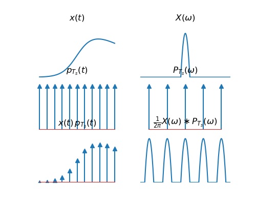
Fig. 5.36 Sampling.

From this figure it is obvious that in case the sampling frequency is more than twice as large as the highest frequency in the signal, i.e. \(\omega_s>2\omega_b\), the shifted copies of the spectrum of the original signal do not overlap. In that case we can reconstruct the original spectrum and from that the original signal.

Important

The sampling theorem states that in case the sampling frequency is more than two times larger than the highest frequency in the signal, the CT signal \(x(t)\) can be exactly reconstructed from its DT samples \(x[n]\).

In the next section we will look at interpolation as the way to reconstruct a CT signal from its DT samples.

In the case that the sampling frequency is below the magic limit of twice the largest frequency in the signal the shifted copie of the original spectrum will overlap and in the summation original high frequencies will emerge at lower frequencies. This effect is called aliasing