5.5.3. Canonical Systems

In classical control theory two systems are the canonical systems: the first and second order systems (higher order systems can be constructed by cascading these canonical systems).

5.5.3.1. First Order Systems

A first order system is characterized with a differential equation having only first order derivatives. Although simple these first order systems are of great importance. E.g. a mass-damper system and a mass heating system are examples of first order systems. And often higher order systems can be approximated with a first order system.

The canonical first order system is characterized with transfer function:

\[H(s) = K \frac{1}{1+\tau s}\]

where \(\tau\) is the time constant of the system and \(K\) is the DC gain of the system.

The impulse response can be derived using the Laplace transform pair

\[e^{-at}u(t) \LTright \frac{1}{a+s}\]

We can rewrite \(H(s)\) as

\[H(s) = K \frac{1}{1+\tau s} = \frac{K}{\tau}\frac{1}{1/\tau + s}\]

and thus the impulse response of a first order system is:

\[h(t) = \frac{K}{\tau} e^{-t/\tau}u(t)\]

To calculate the step response of the first order system we use the fact that the Laplace transform of the unit step equals \(1/s\). And thus the Laplace transform of the step response is

\[\frac{K}{s(1+\tau s)}\]

This Laplace transform is not in our table of common transform pairs. But if we calculate the partial fractions of this we are lookking for factors \(A\) and \(B\) such that

\[\frac{K}{s(1+\tau s)} = K\left(\frac{A}{s} + \frac{B}{1+\tau s}\right)\]

meaning that

\[A(1+\tau s) + Bs = 1\]

leading to \(A=1\) and \(B=-\tau\). So the Laplace transform of the step response equals:

\[\frac{K}{s(1+\tau s)} = K\left( \frac{1}{s} - \frac{\tau}{1+\tau s}\right) = K\left( \frac{1}{s} - \frac{1}{1/\tau+ s}\right)\]

Now we have two terms that are in the table of Laplace transform pairs and the step response of a first order system is:

\[K\left(u(t) - e^{-t/\tau}u(t)\right) = K(1-e^{-t/\tau})u(t)\]

Show code for figure

import numpy as np
import matplotlib.pyplot as plt
from scipy import signal
import control

plt.clf()

tau = 1
H = control.tf([1], [tau, 1])
t, ystep = control.step_response(H)
plt.plot(t, ystep, label=r'$\tau=1$');

tau=2
H = control.tf([1], [tau, 1])
t, ystep = control.step_response(H)
plt.plot(t, ystep, label=r'$\tau=2$');
plt.legend();
plt.savefig('source/figures/firstorder_stepresponse.png')

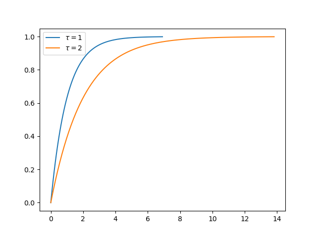
Fig. 5.51 Step Response of First Order System.

5.5.3.2. Second Order Systems

A canonical second order system is characterized with transfer function

\[H(s) = \frac{\w_0^2}{s^2 + 2 \beta \w_0 s + \w_0^2}\]

where \(\w_0\) is the undamped (natural) frequency and \(\beta\) is the damping parameter.

This system has two poles that determine the behaviour of the system. Here study its impulse response and step response.

The poles can be calculated with the quadratic formula:

\[\begin{split}p_{1,2} &= \frac{-2\beta\w_0 \pm \sqrt{4\beta^2\w_0^2 - 4 \w_0^2}}{2}\\ &= -\beta\w_0 \pm \w_0\sqrt{\beta^2-1}\\ &= \w_0\left( -\beta \pm \sqrt{\beta^2-1} \right)\end{split}\]

We can distinguish four different situations depending on the value of \(\beta\).

\(\beta=0\) Undamped

For an undamped system we get:

\[H(s) = \frac{\w_0^2}{s^2+\w_0^2}\]

such that the Laplace transform of the step response equals

\[\frac{H(s)}{s} = \frac{\w_0^2}{s(s^2+\w_0^2)}\]

We want to write this like

\[\frac{A}{s} + \frac{Bs}{s^2+\w_0^2}\]

leading to

\[As^2 + A\w_0^2 + Bs^2 = \w_0^2\]

such that

\[A=1, \quad B=-1\]

The Laplace transform of the step response then becomes:

\[\frac{H(s)}{s} = \frac{1}{s} - \frac{s}{s^2+\w_0^2}\]

From the table of Laplace transform pairs we find the step response of an undamped second order system:

\[\left( 1 - \cos(\w_0 t) \right) u(t)\]

Evidently this is where the term undamped comes from: a step at the input leads to a sinusoidal response with infinite duration.

Show code for figure

import numpy as np
import matplotlib.pyplot as plt
from scipy import signal
import control

plt.clf()

w0 = np.pi
b = 0
t = np.linspace(0, 20, 1000)
H = control.tf([w0**2], [1, 2*b*w0, w0**2])
_, ystep = control.step_response(H, t)
plt.plot(t, ystep, label=r'$\omega_0=\pi$');

w0 = np.pi/2
H = control.tf([w0**2], [1, 2*b*w0, w0**2])
_, ystep = control.step_response(H, t)
plt.plot(t, ystep, label=r'$\omega_0=\pi/2$');
plt.legend();

plt.savefig('source/figures/secondorder_undamped.png')

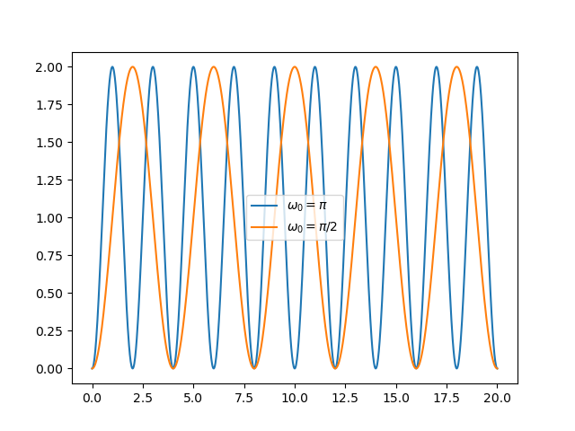
Fig. 5.52 Step Response of Second Order Undamped System.

\(0<\beta<1\) Underdamped

For \(\beta\) in between zero and one the system is underdamped. It will oscillate but the amplitude will decrease over time.

Show code for figure

import numpy as np
import matplotlib.pyplot as plt
from scipy import signal
import control

plt.clf()

w0 = np.pi
t = np.linspace(0, 10, 1000)

for b in [0.20, 0.50]:
   H = control.tf([w0**2], [1, 2*b*w0, w0**2])
   _, ystep = control.step_response(H, t)
   plt.plot(t, ystep, label=r'$\beta={}$'.format(b));

plt.legend();

plt.savefig('source/figures/secondorder_underdamped.png')

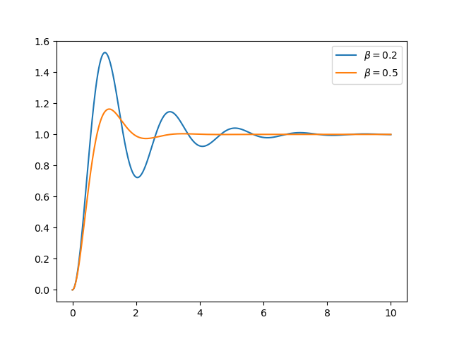
Fig. 5.53 Step Response of Second Order Underdamped System.

\(\beta = 1\) Critically Damped

In case \(\beta=1\) there are two identical real valued poles:

\[p_{1,2} = -\w_0\]

and we can write

\[H(s) = \frac{\w_0^2}{(s+\w_0)(s+\w_0)} = \frac{\w_0}{s+\w_0}\frac{\w_0}{s+\w_0} = \frac{1}{1+s/\w_0} \frac{1}{1+s/\w_0}\]

showing that a critically damped second order system is the cascade of two identical first order system each with time constant \(1/\w_0\).

Show code for figure

import numpy as np
import matplotlib.pyplot as plt
from scipy import signal
import control

plt.clf()
w0 = np.pi
b = 1
t = np.linspace(0, 5, 1000)

H = control.tf([w0**2], [1, 2*b*w0, w0**2])
_, ystep = control.step_response(H, t)
plt.plot(t, ystep, label=r'$\omega=\pi$');

w0 = np.pi/2
H = control.tf([w0**2], [1, 2*b*w0, w0**2])
_, ystep = control.step_response(H, t)
plt.plot(t, ystep, label=r'$\omega=\pi/2$');
plt.legend();

plt.savefig('source/figures/criticallydamped2ndstep.png')

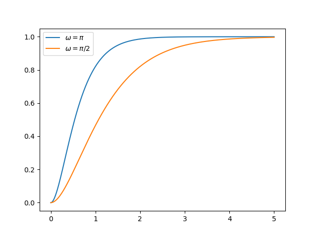
Fig. 5.54 Step Response of Second Order Critically Damped System.

\(\beta>1\) Overdamped

For \(\beta>1\) we have two poles both of which are real valued:

\[p_{1,2} = \w_0\left(-\beta \pm \sqrt{\beta^2-1} \right)\]

Show code for figure

import numpy as np
import matplotlib.pyplot as plt
from scipy import signal
import control

plt.clf()

w0 = np.pi

b = 1
t = np.linspace(0, 10, 1000)

H = control.tf([w0**2], [1, 2*b*w0, w0**2])
_, ystep = control.step_response(H, t)
plt.plot(t, ystep, '--', label=r'$\beta={}$ (critically damped)'.format(b));

b = 2
t = np.linspace(0, 10, 1000)

H = control.tf([w0**2], [1, 2*b*w0, w0**2])
_, ystep = control.step_response(H, t)
plt.plot(t, ystep, label=r'$\beta={}$'.format(b));

b = 4
H = control.tf([w0**2], [1, 2*b*w0, w0**2])
_, ystep = control.step_response(H, t)
plt.plot(t, ystep, label=r'$\beta={}$'.format(b));
plt.legend();


plt.savefig('source/figures/overdamped2ndstep.png')

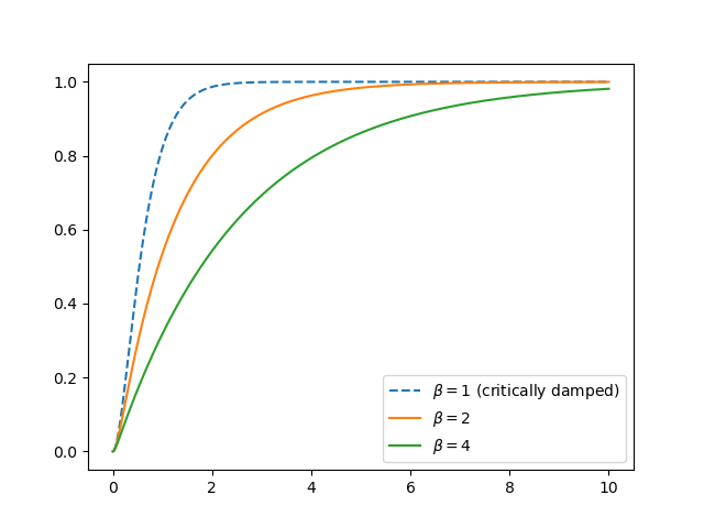
Fig. 5.55 Step Response of Second Order Overdamped System. The critically damped response is shown for comparison.