1.1. Systems

In these lecture notes we restrict ourselves to the most simple systems: SISO systems. Systems with one input signal (Single Input) and one output signal.

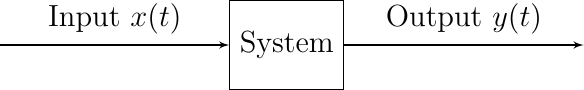
When the system is fed with an input signal \(x(t)\) it outputs the signal \(y(t)\). For now a system is just a black box for us. We will often use the block diagram representation of systems.

Fig. 1.1 A one input, one output (SISO) system

More complex systems have multiple inputs and multiple outputs: MIMO systems.

We will often find the need to use several systems and combine them into a new systems.

Cascaded Systems

Two systems connected in such a way that the output of one system is the input to the second system are cascaded or connected in series.

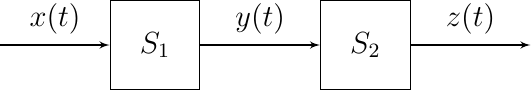
Fig. 1.2 Cascaded (or serial) Systems

Addition / Subtraction

One signal \(x(t)\) can be splitted to function as the input of two systems \(S_1\) and \(S_2\). The output of the two systems can then, for instance, be added together to result in one signal again.

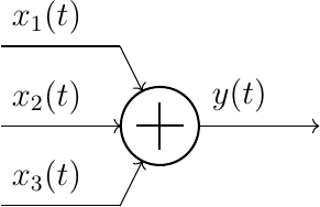
Fig. 1.3 Adding signals. \(y(t) = x_1(t) + x_2(t) + x_3(t)\).

Feedback Loops

When an output signal of a system is fed into the input of the system we talk of a feedback loop. Most often a negative feedback loop is used where the output signal \(y(t)\) is subtracted from the input signal \(x(t)\) and \(x(t)-y(t)\) is fed into the system.

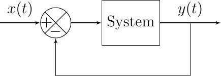
Fig. 1.4 Feedback Loop

The feedback loop will often contain a second system. Feedback loops are very often used in signal processing. We will see examples when building systems for a special purpose and also when discussing classical control systems.

In a later section when we restrict ourselves to linear systems we will look again at the block diagrams to construct composite systems.