5.4.3. IIR Filters in Python
In this section we will take a prototype analog filter and use the bilinear transformation to map it onto a digital filter. The recipe is:
Select or design an analog filter with rational transfer function
\[H(s;\w_0) = \frac{N(s;\w_0)}{D(s;\w_0)}\]where both \(N(s;\w_0)\) and \(D(s;\w_0)\) are polynomials in \(s\). We assume the characteristic defining frequency for this filter is the natural frequency \(\w_0\) (we use \(s;\w_0\) to indicate that \(\w_0\) is a parameter to the transfer function.
Decide on the sampling frequency \(f_s\) that is going to be used in the discrete time domain.
Prewarp the natural frequency
\[\w'_0 = \frac{2}{T_s}\tan\left(\frac{\w_0 T_s}{2}\right)\]then \(H(s;\w'_0)\) is the transfer function that will be used in the bilinear transformation.
The bilinear transformation takes two polynomials \(N(s;\w'_0)\) and \(D(s;\w_0)\) in the s-domain and returns two polynomials \(N(x,\w_0)\) and \(D(z;\w_0)\) in the z-domain that define the transfer function:
\[H(z;\w_0) = \frac{N(z;\w_0)}{D(z;\w_0)}\]for the digital IIR filter.
Working in Python we will use the package scipy.signal. As an example we will look at a second order lowpass filter with \(\w_0=2\pi f_0 = 2\pi 2000\) and \(Q=1\). Following the recipe:
The analog filter:
\[H(s;\w_0) = \frac{\w_0^2}{s^2 + \frac{\w_0}{Q} + \w_0^2}\]with \(\w_0=4000\pi\) and \(Q=1\).
Sampling frequency \(f_s = 44100\)
Pre-warp:
\[\begin{split}\w'_0 &= \frac{2}{T_s}\tan\left(\frac{\w_0 T_s}{2}\right)\\ &= 2 f_s \tan\left( \frac{\w_0}{2 f_s} \right)\\ &= 88200 \tan\left( \frac{4000\pi}{88200} \right) &\approx 12566 \text{ rad/s}\end{split}\]Set
\[H(s; \w'_0) = \frac{N(s; \w'_0)}{D(s;\w'_0)} = \frac{12566^2}{s^2 + \frac{12566}{1}s + 12566^2}\]and with the bilinear transform get
\[H(z) = \frac{N(z)}{D(z)}\]
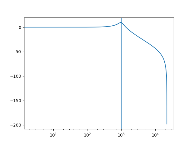
In the code below we follow this recipe in Python using scipy.signal.
Show code for figure
 1import numpy as np
 2import matplotlib.pyplot as plt
 3import scipy.signal as sg
 4
 5plt.close('all')
 6
 7def LP2s(w0, Q):
 8    return [w0**2], [1, w0/Q, w0**2]
 9
10def pre_warp(w0, fs):
11    return 2*fs * np.tan(w0/2/fs)
12
13
14fs = 44100
15w0 = 2 * np.pi * 1000
16
17wa0 = pre_warp(w0, fs)
18
19lp2s = LP2s(wa0, 3)
20
21lp2z = sg.bilinear(*lp2s, fs=fs)
22
23lti_lp2z = sg.dlti(*lp2z, dt=1/fs)
24
25W, H = lti_lp2z.freqresp()
26plt.plot(W*fs/np.pi/2, 20*np.log10(np.abs(H)))
27plt.xscale('log')
28plt.axvline(w0/2/np.pi)
29
30plt.savefig('source/figures/freqresp_LP2.png')
Applying the digital filter lti_lp2z to a signal is easy. The function lfilter takes the nominator, denominator pair in the z-domain and runs the filter over the given input.
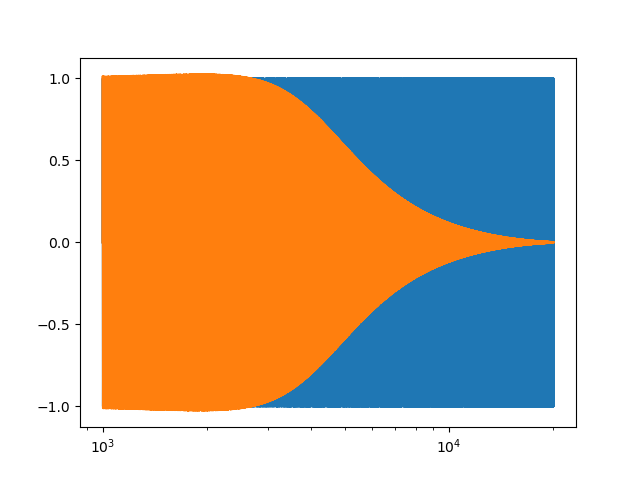
As a test signal we will use a chirp signal that runs from minimal frequency below the natural frequency of our filter to a frequency that is abonve the natural frequency of our filter. This should be a nice indication of the frequency response of the filter.
Show code for figure
 1import numpy as np
 2import matplotlib.pyplot as plt
 3import scipy.signal as sg
 4
 5plt.close('all')
 6
 7def LP2s(w0, Q):
 8    return [w0**2], [1, w0/Q, w0**2]
 9
10def pre_warp(w0, fs):
11    return 2*fs * np.tan(w0/2/fs)
12
13fs = 44100
14w0 = 2 * np.pi * 4000
15wa0 = pre_warp(w0, fs)
16lp2s = LP2s(wa0, 0.8)
17lp2z = sg.bilinear(*lp2s, fs=fs)
18lti_lp2z = sg.dlti(*lp2z, dt=1/fs)
19
20def generate_chirp(startf, endf, fs, duration):
21    """Generate chirp signal."""
22    N = int(duration * fs)
23    t = np.linspace(0, duration, N)
24    phase = 2 * np.pi * (startf * t + (endf - startf) / duration / 2 * t**2)
25    ft = startf + (endf-startf) / duration*t
26    return t, ft, np.sin(phase)
27
28t, ft, x = generate_chirp(1000, 20000, 44100, 5)
29y = sg.lfilter(*lp2z, x)
30plt.plot(ft, x)
31plt.plot(ft, y)
32plt.xscale('log')
33plt.savefig('source/figures/chirpresp_LP2.png')