2.1. Definition and Properties
2.1.1. Linearity and Time Invariance
Let’s consider a one input \(x\) and one output \(y\) system \(\op L\), i.e. \(y = \op L x\). A system is called a linear system in case for a weighted combination of input signals the response is the same weighted combination of the individually processed signals. For the combination of two signals \(x_1\) and \(x_2\) and for any real numbers \(a_1\) and \(a_2\) this means that:
A system \(\op L\) is called time or shift invariant in case \(\op L x_s = (\op L x)_s\) where \(x_s\) denotes the signal \(x\) delayed (shifted) over \(s\), i.e.
For a shift invariant system the order of shifting and applying the system operator \(\op L\) is not important. A linear, time invariant system is often denoted as a LTI system.
Consider a LTI system \(\op L\) with a step response
where \(u(t)\) is the unit step function. Linearity and time invariance makes it easy to calculate the response of the same system to a pulse function of the form:
Note that we can write this pulse function as a linear combination of two shifted step functions:
where \(u\) is the step function. Because of linearity and time invariance the response of the system to this pulse function is:
Show code for figure
 1import numpy as np
 2import matplotlib.pyplot as plt
 3
 4t = np.linspace(0,10,1000)
 5t1 = 3
 6t2 = 6
 7x1 = 1.0*(t>=t1)
 8x2 = 1.0*(t>=t2)
 9x = x1 - x2
10y1 = x1*(1-np.exp(-(t-t1)))
11y2 = x2*(1-np.exp(-(t-t2)))
12y = y1 - y2
13
14fig, axs = plt.subplots(3, 2, sharex=True, sharey=True)
15
16axs[0,0].plot(t,x1,'b',lw=3)
17axs[0,0].set_title(r'$u(t-t_1)$')
18
19axs[1,0].plot(t,x2,'b',lw=3)
20axs[1,0].set_title(r'$u(t-t_2)$')
21
22axs[2,0].plot(t,x,'b',lw=3)
23axs[2,0].set_title(r'$x(t)$')
24
25axs[0,1].plot(t,y1,'g',lw=3)
26axs[0,1].set_title(r'$y_1(t)$')
27
28axs[1,1].plot(t,y2,'g',lw=3)
29axs[1,1].set_title(r'$y_2(t)$')
30
31axs[2,1].plot(t,y,'g',lw=3)
32axs[2,1].set_title(r'$y(t)$')
33
34plt.savefig('source/figures/broadpulseresponse.png')
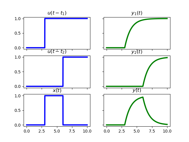
Fig. 2.6 Linear Superposition.
2.1.2. Stable Systems
A system is called a stable system in case a finite change in the input causes a finite change in the output.
Examples of unstable systems:
a ball on top of an sphere. In theory you can put the small ball on the top of the sphere such that its center gravity is right above the center of the sphere. Then the ball will be at rest. But only the slightest push will let the ball drop down from the sphere.
imagine a microphone connected to an amplifier and the amplifier connected to a speaker. The sound from the microphone is amplified and then can be heard from the speaker. Stand in front of the speaker with the microphone and you will realize that this is not a stable system.
Stability is most often a desirable property of a system. We return to stability when we discuss the design of filters (another word for a one input one output systems) and when discussing control theory.
2.1.3. Causal Systems
A system is causal in case in case the output at time \(t\), i.e. \(y(t)\) does not depend on the input values at times \(u>t\). This is of course a requirement for any system that processes signal ‘live’, we then don’t know what is coming in the future and we can only use the past to make up the output value.
Especially for signals that vary in time causality is an import requirement in practice. For spatial signals (images) the requirement for causality is without meaning as there is no causal ordering of the pixels in an image.