4.2.5. The Z-Operator

\(\newcommand{\op}[1]{\mathsf #1}\) \(\newcommand{\ztarrow}{\stackrel{\op Z}{\longrightarrow}}\) \(\newcommand{\z}{\op z}\)

The Z-transform takes a sequence \(x[n]\) and returns a function \(X(z)\). In the z-domain we have seen that shifting a signal \(x[n]\) over \(n_0\), resulting in \(x[n-n_0]\), leads to the Z-transform \(z^{-n_0}X(z)\) where \(X(z)\) is the transform of the original signal.

This observation has lead to the introduction of the \(\z\)-operator that takes a discrete signal \(x\) and shifts it:

\[(\z x)[n] = x[n-1]\]

With this algebraic notation of a shift, together with multiplications and summations this is all we need to characterize /all/ linear translation invariant filters.

Note that shifting over 3 samples corresponds with the operator \(\z \z \z = \z^3\) or in general:

\[(\z^{m} x)[n] = x[n-m]\]

Evidently the operator \(\z^{-1}\) corresponds with a shift in the opposite direction and thus the above equation may be interpreted for both positive and negative (integer) values of \(m\).

A simple non-causal running average filter over 5 samples can be defined as the operator:

\[\op f = \tfrac{1}{5}\left( \z^2 + \z^1 + 1 + \z^{-1} + \z^{-2}\right)\]

Using this filter to process a signal \(x\) is denoted as \(\op f x\) or \(\op f(x)\) where we assume \(x\) is a discrete signal.

A recursive band stop filter is defined with:

\[y[n] = 1.8 y[n-1] - 0.9 y[n-2] + x[n] - 1.9 x[n-1] + x[n-2]\]

Using the \(\z\) operator we may write:

\[y[n] = 1.8 (\z^{-1} y)[n] - 0.9 (\z^{-2}y)[n] + x[n] - 1.9 (\z^{-1}x)[n] + (\z^{-2}x)[n]\]

because now all signals are indexed at \(n\) we may leave the index out to obtain the expression that is valid for all \(n\):

\[y = 1.8 \z^{-1} y - 0.9 \z^{-2}y + x - 1.9 \z^{-1}x + \z^{-2}x\]

or equivalently:

\[y = \frac{1 - 1.9 \z^{-1} + \z^{-2}}{1 - 1.8 \z^{-1} + 0.9 z^{-2}} x = \frac{\z^2-1.9\z+1}{\z^2-1.8\z+0.9} x\]

This band stop filter thus can be formally defined as:

\[\op f = \frac{\z^2-1.9\z+1}{\z^2-1.8\z+0.9}\]

and of course in the definition of the filter \(\op f\) you recognize the Z-transform of the impulse response of the filter characterized with the Z-transform:

\[H(z) = \frac{z^2-1.9z+1}{z^2-1.8z+0.9}\]

Please note however that \(H(z)\) is not the filter \(\op f\). In the expression for \(H(z)\), \(z\) is a complex number whereas in the expression for \(\op f\), \(\z\) is an operator. The operator notation for \(\op f\) is a symbolic notation. It can be implemented in practice using the difference equation we started with.

Using the \(\z\) operator to define discrete LTI filters is nowadays often used. In fact even software is written in which the \(\z\) operator notation plays a central role. Below we give some examples using the ‘audiolazy’ Python package.

import numpy as np
import matplotlib.pyplot as plt
from audiolazy import z

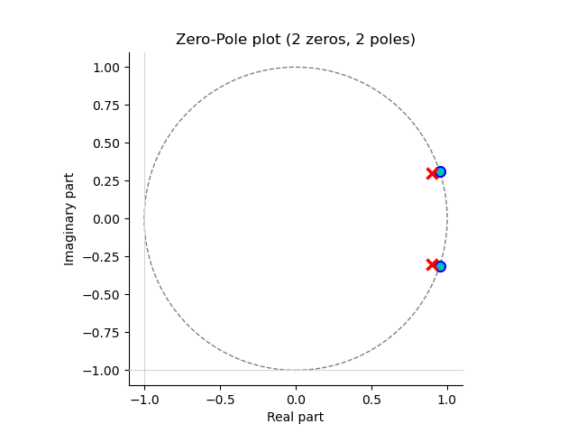
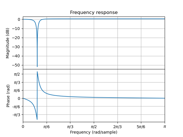
H = (z**2-1.9*z+1)/(z**2-1.8*z+0.9);
H.zplot().savefig('source/figures/hzplot.pdf');
H.plot().savefig('source/figures/hfplot.pdf');

Note that in the code given here the function savefig() is used to save the figure in a file. In an interactive session you can use show() instead.

Although conceptually nice, audiolazy still lacks soms of the standard filters. A lot of these standard filters are available in scipy.signal. In the lecture notes on filter design some examples of the use of scipy will be given.

Todo

look at the status of audiolazy