2.3. Linear Discrete Time Systems

We have seen that the working of any LTI system, continuous or discrete time, is completely characterized as a convolution with its impulse response.

For discrete time systems that are often implemented in software, the convolution thus seems the logical way to implement such a system (or filter as we will call it). But for discrete time systems there is another way of characterizing and implementing a class of LTI systems, namely through the use of difference equations.

Consider an input-output relation specified as:

$$a_0 y[n] + a_1 y[n-1] + \cdots + a_N y[n-N] = b_0 x[n] + b_1 x[n-1] + \cdots + b_M x[n-M]$$

or

(2.1) $$\sum_{k=0}^N a_k y[n-k] = \sum_{k=0}^M b_k x[n-k]$$

This expression for the difference equation easily leads to the conclusion that the system described is indeed an LTI system.

Setting $a_0=1$ (which of course can be done by dividing the above expression by $a_0$) we can rewrite in the form:

$$y[n] = \sum_{k=0}^M b_k x[n-k] - \sum_{k=1}^N a_k y[n-k]$$

this is a recipe for calculating $y[n]$ as a linear combination of $x[n],\ldots,x[n-M]$ and of $y[n-1],\ldots,y[n-N]$. I.e. to calculate $y[n]$ we use values of the input signal but also of the output signal that we have already calculated.

Consider the following example:

$$y[n] = x[n] + \alpha y[n-1]$$

Because the difference equation described an LTI system, it should also be characterized with its impulse response funtion $h[n]$. Note that $h[n]$ is the response $y[n]$ given the impulse as input $x[n]=\delta[n]$.

Assuming $y[-1]=0$ we get:

$$\begin{split}h[0] &= 1\\ h[1] &= \alpha\\ h[2] &= \alpha^2\\ \vdots\\ h[n] &= \alpha^n\end{split}$$

Note that the impulse response is non zero for all $n\geq 0$. This is called an infinite impulse response filter. Evidently this filter is only stable in case $|\alpha|<1$.

Show code for figure

import numpy as np
import matplotlib.pyplot as plt

plt.clf()
n = np.arange(32)
h = 0.8**n
plt.stem(n, h, use_line_collection=True);

plt.savefig('source/figures/iir_simple_1.png')

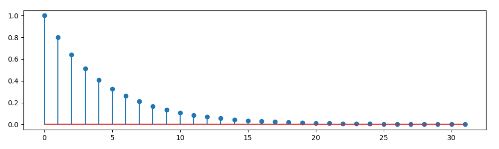
Fig. 2.10 Infinite impulse response: $h[n]=0.8^n u[n]$

For a negative value for $\alpha$ we get a totally different linear system.

Show code for figure

plt.clf()
n = np.arange(32)
h = (-0.8)**n
plt.stem(n, h, use_line_collection=True);

plt.savefig('source/figures/iir_simple_2.png')

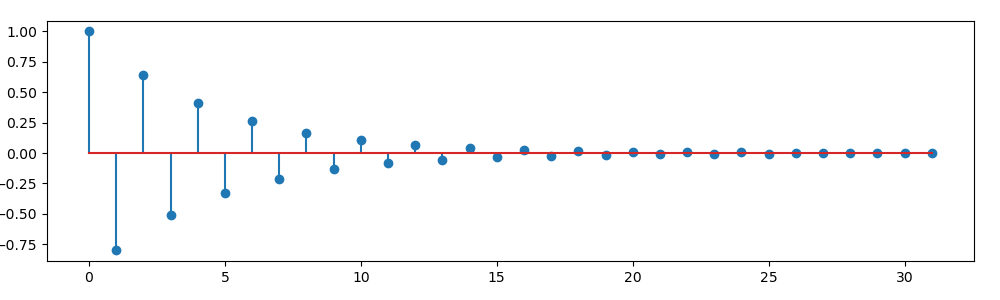
Fig. 2.11 Infinite impulse response: $h[n]=(-0.8)^n u[n]$

In this section we won’t look at these IIR filters but come back to this subject in the section of filters after we have discussed the Z-transform.