4.1.4. Differential Equations and the Laplace Transform

\(\newcommand{\dfdt}[2]{\frac{d^{#1} #2}{d t^{#1}}}\)

The Laplace transform is an important mathematical tool to solve differential equations. Many physical systems with input \(x(t)\) and output \(y(t)\) can be physically modelled with a differential equation of the form:

\[a_N \dfdt{N}{y(t)} + \cdots + a_1 \dfdt{}{y(t)} + a_0 y(t) = b_M \dfdt{M}{x(t)} + \cdots + b_1 \dfdt{}{x(t)} + b_0 x(t)\]

Applying the Laplace transform om both sides of the equation we get

\[\LT\left\{a_N \dfdt{N}{y(t)} + \cdots + a_1 \dfdt{}{y(t)} + a_0 y(t)\right\} = \LT\left\{b_M \dfdt{M}{x(t)} + \cdots + b_1 \dfdt{}{x(t)} + b_0 x(t)\right\}\]

Due to the linearity of the Laplace transform:

\[\begin{split}a_N\LT\left\{\dfdt{N}{y(t)}\right\} + \cdots + a_1 \LT\left\{\dfdt{}{y(t)}\right\} + a_0 \LT\left\{y(t)\right\} =\\ b_M\LT\left\{\dfdt{M}{x(t)}\right\} + \cdots + b_1 \LT\left\{\dfdt{}{x(t)}\right\} + b_0 \LT\left\{x(t)\right\}\end{split}\]

and using the property for the Laplace transform for n-th order derivatives we arrive at

\[a_N s^N Y(s) + \cdots + a_1 s Y(s) + a_0 Y(s) = b_M s^M X(s) + \cdots + b_1 s X(s) + b_0 X(s)\]

or

\[\left(a_N s^N + \cdots + a_1 s + a_0\right) Y(s) = \left(b_M s^M + \cdots + b_1 s + b_0\right) X(s)\]

The transfer function of this system then equals:

\[H(s) = \frac{Y(s)}{X(s)} = \frac{b_M s^M + \cdots + b_1 s + b_0}{a_N s^N + \cdots + a_1 s + a_0} = \frac{\sum_{m=0}^{M} b_m s^m}{\sum_{n=0}^{N} a_n s^n}\]

4.1.4.1. Poles and Zeros in the S-plane

Consider a generic transfer function in the s-domain:

\[H(s) = \frac{\sum_{m=0}^{M} b_m s^m}{\sum_{n=0}^{N} a_n s^n}\]

Note that for any \(n\)-th order complex polynomial with real coefficients we have exactly \(n\) roots (possible multiples). Thus we may rewrite the transfer function as:

\[H(s) = K \frac{\prod_{m=0}^{M} (s-z_m)}{\prod_{n=0}^{N} (s-p_n)}\]

where the \(z_m\)’s are the zeros (the roots of the numerator) and the \(p_n\)’s are the poles (the roots of the denominator). The factor \(K\) is needed to compensate for the fact that in the original expression of \(H\) the coefficient for the highest power is not necessarily equal to one.

Without proof we state that:

1. For a system with real coefficients in the differential equation the poles and zeros come in conjugate pairs or lie on the real axis.

2. For a system with transfer function \(H\) the poles should lie in the left half of the s-splane for the system to be a stable system.

3. And remember the Fourier transform in the s-plane is ‘found’ along the imaginary axis.

4.1.4.2. An Electronic Example

In an appendix on analog electronics the voltage \(u(t)\) over a capacitor and the current \(i(t)\) through the capacitor are linked as:

\[i(t) = C \frac{d u(t)}{dt}\]

It is the physical modeling that leads to a differential equation that ‘fits’ the Laplace transform:

\[I(s) = s C U(s)\]

Consider a capacitor in series with a loudspeaker (which in good approximation operates as if it were a resistor) as show in the figure below.

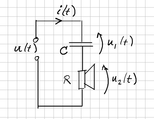
Fig. 4.1 A tweeter (a speaker driver optimized to reproduce the high frequencies) is protected from too low frequencies by a capacitor that is in series with the speaker.

Physics tells us:

\[\begin{split}u(t) &= u_1(t) + u_2(t)\\ i(t) &= C \frac{d u_1(t) }{dt}\\ u_2(t) &= i(t) R\end{split}\]

The Laplace transform is used to make this into an algebraic set of equations:

\[\begin{split}U(s) &= U_1(s) + U_2(s)\\ I(s) &= s C U_1(s)\\ U_2(s) &= R I(s)\end{split}\]

We are interested in the voltage \(u_2(t)\) in relation to the input voltage \(u(t)\). The transfer function for the electronic circuit is:

\[H(s) = \frac{U_2(s)}{U(s)} = \frac{RCs}{1+RCs}\]

Again let’s consider the asymptotic behavior of the magnitude of the transfer function in the frequency domain to obtain a qualitative insight into this circuit.

The Fourier transform is obtained from the s-domain transfer function by substituting \(s=j\w\). So:

\[H(\w) = \frac{jRC\w}{1+jRC\w}\]

and thus

\[|H(\w)| = \frac{RC\w}{\sqrt{1+R^2C^2\w^2}}\]

We consider the two cases:

1. \(RC\w\ll 1\), then \(|H(\w)| \approx RC\w\), and

2. \(RC\w\gg 1\), then \(|H(\w)| \approx 1\).

Observe that these two asymptotic approximations intersect at the cut-off frequency \(\w_c = \frac{1}{RC}\). In decibels we get as asymptotic behavior:

\[\begin{split}20 \log_{10} |H(\w)| = \begin{cases} \log_{10}(RC) + \log_{10}(\w) &: \w < \w_c\\ 0 &: \w\geq \w_c \end{cases}\end{split}\]

So this circuit acts as a high pass filter.

In scipy.signal we can easily define an LTI system in the s-domain. This is illustrated in the code below where a low-pass filter is defined with cut-off frequency at 2000Hz.

import numpy as np
import matplotlib.pyplot as plt
import scipy.signal as sig

fc = 2000
wc = 2 * np.pi * fc
H = sig.lti([1/wc, 0], [1/wc, 1])

f = np.logspace(1, 5, 1000)
w = 2 * np.pi * f
_, magH = H.freqresp(w)
plt.plot(f, 20 * np.log10(np.abs(magH)))
plt.xscale('log')
plt.axvline(fc)

plt.savefig('source/figures/lowpass_response.png')

4.1.4.3. A Mechanical Example

In this subsection we give a simple example of a mass-spring-damper system. It is much like the car suspension example from the chapter on control theory (but somewhat more simple). Consider the following system as sketched in the figure below.

Fig. 4.2 A simple mass-spring-damper system. A block of mass \(M\) slides (friction free) over a surface and is restricted on the right by a spring with constant \(K\) and on the left by a damper with constant \(B\).

This example is simple enough to be able to tackle comfortably with a simple Newtonian view that \(F=ma\) where \(F\) is the total force exerted on the mass \(M\) being the sum of the external force \(f(t)\) directly exerted on the mass, the spring force being exerted when the spring is being pressed (force is proportional to the displacement) and the damper force (that is a function of the speed of movement). The total force balance is:

\[f(x) - K x(t) - B\frac{d x}{dt} = M \frac{d^2 x}{dt^2}\]

where:

\[\begin{split}f(x) &: \text{the external force}\\ -K x(t) &: \text{the spring force}\\ \frac{dx}{dt} &: \text{the velocity}\\ -B\frac{dx}{dt} &: \text{the damper force}\\ M &: \text{the mass}\\ \frac{d^2x}{dt^2} &: \text{the acceleration}\end{split}\]

We consider the external force \(f(t)\) to be the input to the system and the displacement \(x(t)\) the output of the system. Applying the Laplace transform on both sides of the equation we get:

\[F(s) - k X(s) - s B X(s) = s^2 M X(s)\]

Rearranging terms we can write the transfer function \(H(s) = X(s)/F(s)\) as:

\[H(s) = \frac{X(s)}{F(s)} = \frac{1}{M s^2 + B s + K}\]

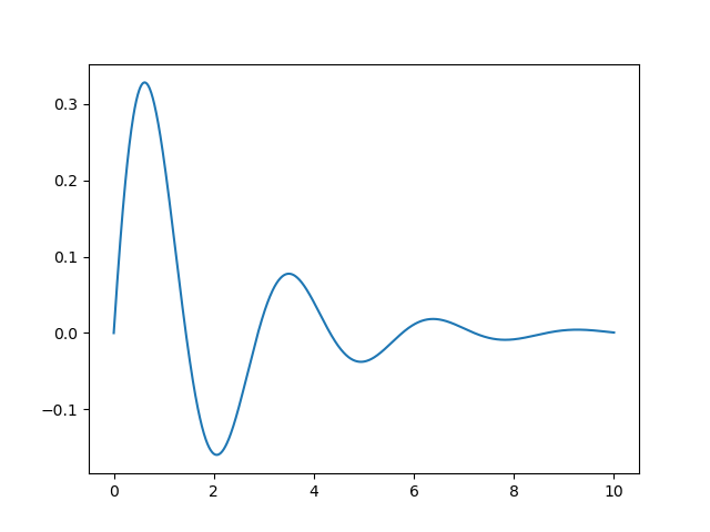
Now imagine that the system is in rest at \(t=0\) and at that time you hit the mass with a massive hammer. That is the physical equivalent of feeding our system with an impulse response.

Evidently the impulse response can be calculated as the inverse Laplace transform of the transfer function \(H(s)\). The practical way to do that is by looking at the table of Laplace transform pairs and see which of the Laplace transforms (almost) matches the given one. Then you have to rewrite the given transfer function to match exactly giving you also the impulse transform. Not in all cases this is possible. Sometimes partial fraction expansion will be needed to write the given transfer function as a sum of functions in the s-domain for which an inverse can be found in the table.

We leave calculating the impulse response as an exercide to the reader.

Another way of visualizing the impulse response is by numerical calculations. In scipy.signal we can easily define transfer functions as rational functions in the s-domain. Then the impulse and step response can be calculated numerically. Look at the code used to draw the impulse and step response of the mass-spring-damper system (assuming \(M=1, B=1, K=5\)).

import numpy as np
import matplotlib.pyplot as plt
import scipy.signal as sig

plt.close('all')

M = 1
B = 1
K = 5
H = sig.lti([1], [M, B, K])

t = np.linspace(0, 10, 1000)
_, h = H.impulse(T=t)

plt.plot(t, h)

plt.savefig('source/figures/impulse_response.png')

We may also visualize the step response of this system. That is when you exert a constant force \(F\) on the mass (think of a propellor mounted on top) that starts at time \(t=0\).

import numpy as np
import matplotlib.pyplot as plt
import scipy.signal as sig

plt.close('all')

M = 1
B = 1
K = 5
H = sig.lti([1], [M, B, K])

t = np.linspace(0, 10, 1000)
_, ur = H.step(T=t)

plt.plot(t, ur)

plt.savefig('source/figures/step_response.png')

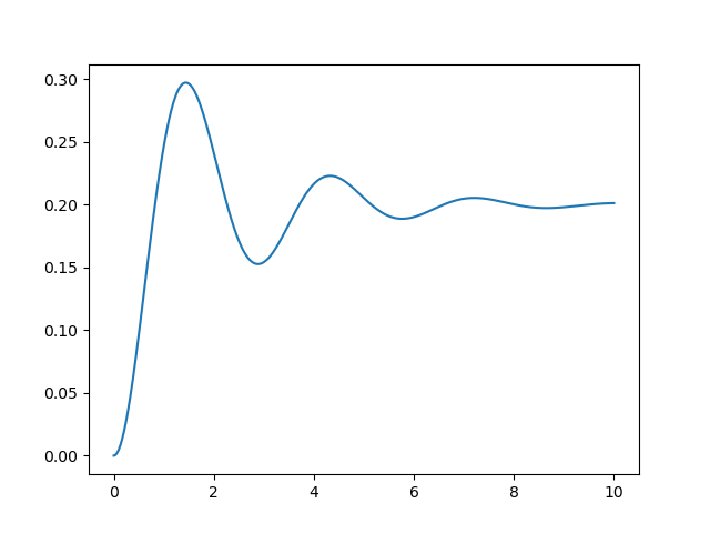
Note that the steady state (for \(t\rightarrow\infty\)) is 0.2 which is to be expected given that at that time the mass is not moving anymore (so the damper does not exert a force) and when the spring is pressed over a distance of 20 cm it exerts a force of 1 Newton (due to the spring constant \(K=5\)) balancing the force of the propellor.

The observed behavior is typical for a second order system. In the chapter on control theory we will look at these types of systems in more detail.