5.4.1. Analog Filters

5.4.1.1. Ideal Filters

Often used ideal filters are illustrated in the figure below and described below the figure.

Show code for figure

import numpy as np
import matplotlib.pyplot as plt
import scipy.signal as sig

plt.close('all')
fig, axs = plt.subplots(2, 2, sharex=True, sharey=True)

w = np.logspace(1,5,1000);
Hlp = 1.0*(w<1000)

axs[0, 0].plot(w, Hlp, linewidth=3)
axs[0, 0].set_ylim(-0.1, 1.1)
axs[0, 0].set_xscale('log')
axs[0, 0].set_title('Low Pass')

Hhp = w>1000
axs[0, 1].plot(w, Hhp, linewidth=3)
axs[0, 1].set_ylim(-0.1, 1.1)
axs[0, 1].set_title('High Pass')

Hbp = 1.0 * np.logical_and(w>500, w<5000)
axs[1, 0].plot(w, Hbp, linewidth=3)
axs[1, 0].set_xlabel(r'$\omega$')
axs[1, 0].set_ylim(-0.1, 1.1)
axs[1, 0].set_title('Band Pass')


Hbr = 1.0 * np.logical_or(w<500, w>5000)
axs[1, 1].plot(w, Hbr, linewidth=3)
axs[1, 1].set_xlabel(r'$\omega$')
axs[1, 1].set_ylim(-0.1, 1.1)
axs[1, 1].set_title('Band Reject')

plt.savefig('source/figures/idealfilters.png')

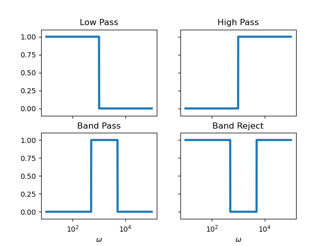
1. Low pass filter. Frequencies below the cut-off frequencies are passed through without change and frequencies higher than \(\w_c\) are not passed at all.

2. High Pass Filter. The frequencies above the cut-off are passed through unchanged.

3. Band Pass Filter. The frequencies in the interval from a lower frequency up to higher frequency are passed through.

4. Band Reject Filter. The frequencies in the interval are not passed at all. In practical applications a band reject filter is often designed to suppress one specific frequency. Such a very narrow band filter is called a notch filter.

All these filter are indeed ideal filters. They cannot be realized in physical hardware. All analog filters are therefore approximations of the ideal filters. That is why there is no best design for a filter. It all depends on the use of the filter.

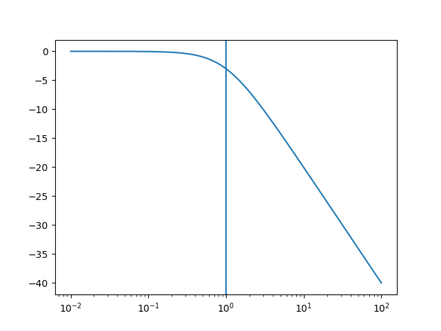
5.4.1.2. The Canonical (Low Pass) First Order Filter and its Transformations

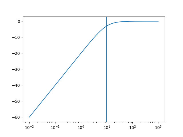
The canonical low-pass first order analog filter is given by the following transfer function in the s-domain.

\[H(s) = \frac{1}{1+s}\]

The frequency response is

\[H(\w) = \frac{1}{1+j\w}\]

A plot of \(|H(\w)|\) in dB and a logarithmic frequency axis shows:

Show code for figure

import numpy as np
import matplotlib.pyplot as plt
import scipy.signal as sig

plt.close('all')

H = sig.lti([1], [1, 1])


w, magH = H.freqresp(np.logspace(-2,2,1000))
plt.plot(w, 20 * np.log10(np.abs(magH)))
plt.xscale('log')
plt.axvline(1)

plt.savefig('source/figures/canonical_lowpass.png')

5.4.1.2.1. Selecting the Corner Frequency

The cut-off frequency of our canonical low pass filter is 1. We can ‘shift’ this to any desired value, say \(\w_c\) with

\[H(s) = \frac{1}{1+\frac{s}{\w_c}}\]

Evidently we are not really shifting the response as we are scaling the frequency axis. However scaling the linear frequency axis corresponds with a shift on the logarithmic frequency axis. Indeed we have a ‘shifted’ frequency response.

Show code for figure

import numpy as np
import matplotlib.pyplot as plt
import scipy.signal as sig

plt.close('all')

H = sig.lti([1], [1, 1])
w, magH = H.freqresp(np.logspace(-2,3,1000))
plt.plot(w, 20 * np.log10(np.abs(magH)), c='grey', label=f'$\omega_c=1$')
plt.xscale('log')
plt.axvline(1, c='grey')

wc=10
H = sig.lti([1], [1/wc, 1])
w, magH = H.freqresp(np.logspace(-2,3,1000))
plt.plot(w, 20 * np.log10(np.abs(magH)), label=f'$\omega_c=10$')
plt.xscale('log')
plt.axvline(wc)

plt.legend()

plt.savefig('source/figures/canonical_lowpass_wc.png')

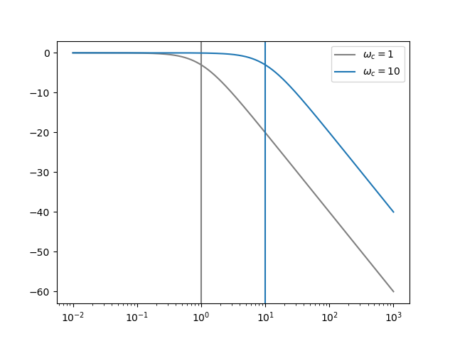
So starting from a canonical low pass filter the substitution

\[s\rightarrow \frac{s}{\w_c}\]

‘shifts’ the cut-off frequency to \(\w_c\).

The canonical low-pass filter is easily build with passive electronic components. Consider the following simple circuit of an inductor in series with a resistor,

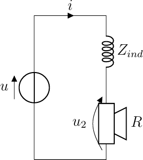
The voltage over the resister as a function of the voltage over both components is (in the s-domain):

\[H(s) = \frac{U_2(s)}{U(s)} = \frac{R}{R+sL} = \frac{1}{1+s\frac{L}{R}}\]

We see this is indeed the transfer function of a low pass filter

5.4.1.2.2. From Low Pass to High Pass

From the canonical low pass filter we can construct the high pass filter with cut-off frequency \(\w_c\) by the substitution

\[s \rightarrow \frac{\w_c}{s}\]

leading to:

\[H(\w) = \frac{1}{1+\frac{\w_c}{s}} = \frac{s}{s+\w_c}\]

Show code for figure

import numpy as np
import matplotlib.pyplot as plt
import scipy.signal as sig

plt.close('all')

wc = 10
H = sig.lti([1, 0], [1, wc])


w, magH = H.freqresp(np.logspace(-2,3,1000))
plt.plot(w, 20 * np.log10(np.abs(magH)))
plt.xscale('log')
plt.axvline(wc)

plt.savefig('source/figures/canonical_highpass.png')

5.4.1.2.3. From Low Pass to Bandpass

The easiest way to construct a bandpass filter is to use a low pass filter (with corner frequency \(\w_H\)) and a high pass filter (with corner frequency \(\w_L\)). The cascade (concatenation) of these two filters passes all frequencies in the interval from \(\w_L\) to \(\w_H\).

If we take the first order canonical filters for lowpass and highpass we arrive at the following transfer function for a band pass filter:

\[H(s) = \frac{\w_H s}{s^2 + (\w_L + \w_H)s + \w_h\w_L}\]

Show code for figure

import numpy as np
import matplotlib.pyplot as plt
import scipy.signal as sig

plt.close('all')

wL = 1
wH = 100
H = sig.lti([wH, 0], [1, wL+wH, wL*wH])

w, magH = H.freqresp(np.logspace(-2,3,1000))
plt.plot(w, 20 * np.log10(np.abs(magH)))
plt.xscale('log')
plt.axvline(wL)
plt.axvline(wH)
# plt.axhline(0)
# plt.axhline(-3)

plt.savefig('source/figures/bandpass.png')

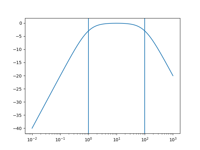
Fig. 5.38 Bandpass Filter parameterized by the low corner frequency \(\w_L\) and high corner frequency \(\w_H\).

We would like our bandpass filter to have unity gain (or 0 dB) for the frequency in the middle of the pass band. The middle frequency is \(\w_0 = \sqrt{\w_L \w_H}\). This is the geometric mean and on a logarithmic scale it is indeed in the middle. It can be shown that

\[| H(\w_0) | = \frac{\w_H}{\w_L + \w_H}\]

So multiplying with the reciproke we arrive at a bandpass filter with unity gain in the (geometric) center of pass band:

\[\begin{split}H(s) &= \frac{\w_L + \w_H}{\w_H} \frac{\w_H s}{s^2 + (\w_L + \w_H)s + \w_h\w_L}\\ &= \frac{(\w_L+\w_H) s}{s^2 + (\w_L + \w_H)s + \w_h\w_L}\end{split}\]

It can be shown that the same bandpass transfer function can be directly obtained from the canonical low pass filter through the substitution

\[s \rightarrow \frac{s^2+\w_0^2}{B s}\]

where \(s_0\) is the center frequency of the pass band and \(B\) is proportional to the width of the pass band. This is the transform that the scipy.signal.lp2bp function from Scipy implements.

We leave it as an exercise to the reader to express the two parameters \(\w_0\) and \(B\) as function of the \(\w_L\) and \(\w_H\) frequencies.

5.4.1.3. Second Order Filters

The easiest way to make a second order filter is to make a cascade of two first order filters. Take the canonical low pass filter with \(\w_c\) as cut-off frequency:

\[H_{LP}(s) = \frac{1}{1+\frac{s}{\w_c}}\]

Cascading two of these filters leads to a total transfer function

\[H_{LP2}(s) = \frac{\w_c^2}{s^2 + 2 \w_c s + \w_c^2}\]

Show code for figure

import numpy as np
import matplotlib.pyplot as plt
import scipy.signal as sig

plt.close('all')


wc=10
H1 = sig.lti([1], [1/wc, 1])
w, magH = H1.freqresp(np.logspace(-2,3,1000))
plt.plot(w, 20 * np.log10(np.abs(magH)), 'b', label=f'First order $\omega_c=10$')
plt.xscale('log')
plt.axvline(wc, c='blue')

H2 = sig.lti([wc**2], [1, 2 * wc, wc**2])
w, magH = H2.freqresp(np.logspace(-2,3,1000))
plt.plot(w, 20 * np.log10(np.abs(magH)), 'r', label=f'Second order $\omega_c=0.64$')
plt.xscale('log')
plt.axvline(np.sqrt(np.sqrt(2)-1) * wc, c='red')
plt.axhline(-3, c='black')

plt.legend()

plt.savefig('source/figures/order2_lowpass_wc.png')

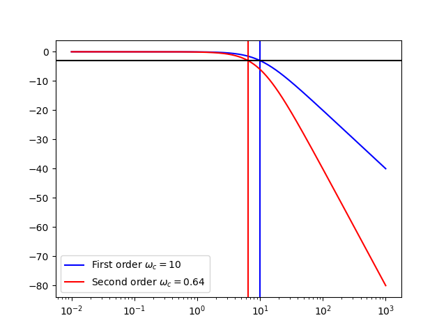
Fig. 5.39 Second Order Low Pass Filter made as the cascade of two identical first order low pass filters. The black horizontal line is the line at -3db defining the cut of frequency. The blue vertical line is the cut off frequency of the first order low pass filter, the red vertical line is at the cut off frequency of the second order filter.

Observe from the above figure:

• The response falls off with 12 dB per octave, i.e. twice as much as the first order low pass filter.

• The frequency \(\w_c\) is not the cutt off frequency of this second order filter (it is the cutt off frequency of the first order filter) The cut off frequency can be calculated to be \(\w_c / \sqrt{\sqrt{2}-1}\).

Cascading two first order filters is not the only way to define a second order filter. For a first order filter the poles by necessity are on the real axis in the s-plane. In general we can make a second order filter where the poles form a conjugate pair. E.g.

\[H_2(s) = \frac{K}{(s-p)(s-p^*)}\]

The pole \(p\) in polair form can be written as:

\[p = r e^{j\phi}\]

without loss of generality we assume that \(p\) is in the quadrant of complex space where \(\Re(p)<0\) (i.e. causal system) and \(\Im(p)\geq 0\). This is equivalent with

\[\begin{split}&r > 0\\ \half\pi < &\phi \leq \pi\end{split}\]

The transfer function than is

\[\begin{split}H_2(s) &= \frac{K}{(s-r e^{j\phi})(s-r e^{-j\phi})}\\ &= \frac{K}{s^2 - 2 r \cos(\phi) s + r^2}\end{split}\]

In order to have unit response for \(H_2(\w)=H_2(s)\Bigr|_{s=j\w}\) for \(\w=0\) we set \(K=r^2\) and obtain:

\[H_2(s) = \frac{r^2}{s^2 - 2 r \cos(\phi) s + r^2}\]

Observe that for \(\phi=\pi\) this second order filter is the same as the low pass filter obtained by cascading two first order low pass filters each with cut-off frequency \(\w_c=r\).

Not let’s vary \(\phi\) and see what the influence is on the frequency response of this filter.

Show code for figure

import numpy as np
import matplotlib.pyplot as plt
import scipy.signal as sig

plt.close('all')

def H2(r, phi):
    return [[r**2], [1, - 2 * r * np.cos(phi), r**2]]

r=10
phis = np.linspace(np.pi/2, np.pi, 6)
for phi in phis:
   H = sig.lti(*H2(r, phi))
   w, magH = H.freqresp(np.logspace(-1,3,1000))
   plt.plot(w, 20 * np.log10(np.abs(magH)), label=f'$\phi = {phi/np.pi:5.2f}\pi$')

plt.xscale('log')
plt.axvline(r, c='blue')

plt.legend()

plt.savefig('source/figures/order2_lowpass_phis.png')

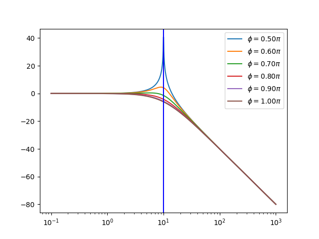
Fig. 5.40 Generic Second Order Low Pass Filters. For all filters we have set \(r=10\). For \(\phi=\pi\) the filter is equivalent to two first order filters with cut-off frequency \(\w_c=r\).

Observe from the figure:

• by varying the value of \(\phi\) we can change the behavior (in the frequency response). Changing the value of \(\phi\) to a lower value than \(\pi\) the frequency response is increased at the frequency \(r\). When \(\phi=\pi/2\) the system becomes (marginally) unstable as seen from the figure where the frequency response jumps to \(\infty\).

• the frequency \(\w=r\) is not the cut-off frequency for this filter. This frequency is however a key parameter for this (family of) filters and is called its natural frequency \(\w_0\).

A more common parameterization of this family of filters is:

\[H_2(s) = \frac{\w_0^2}{s^2 + \frac{\w_0}{Q} s + \w_0^2}\]

where \(\w_0\) is the natural frequency and \(Q\) is the quality factor. In control theory we will see another parameterization:

\[H_2(s) = \frac{\w_0^2}{s^2 + 2\zeta s + \w_0^2}\]

where \(\zeta\) is the damping factor.

So now we have found are canonical second order low pass filter (with \(\w_0=1\)):

\[H_2(s) = \frac{1}{s^2 + \frac{s}{Q} + 1}\]

we can use the transformations discussed previously to obtain a high pass filter or bandpass filter.

5.4.1.3.1. From Low Pass to High Pass

The substitution

\[s \rightarrow \frac{w_0}{s}\]

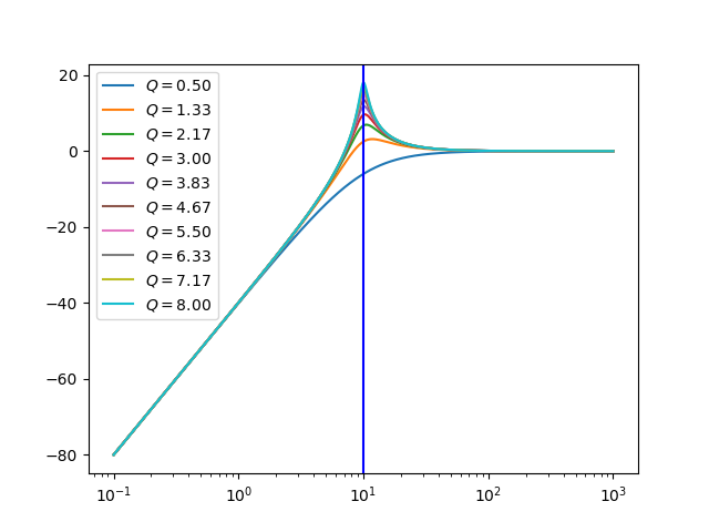
turns a low pass filter into a highpass filter:

\[H(s) = \frac{s}{s^2 + \frac{w_0}{Q} s + 1}\]

Show code for figure

import numpy as np
import matplotlib.pyplot as plt
import scipy.signal as sig

plt.close('all')

def H2(w0, Q):
    return [[1, 0, 0], [1, w0 / Q, w0**2]]

w0=10
Qs = np.linspace(0.5, 8, 10)
for Q in Qs:
   H = sig.lti(*H2(w0, Q))
   w, magH = H.freqresp(np.logspace(-1,3,1000))
   plt.plot(w, 20 * np.log10(np.abs(magH)), label=f'$Q = {Q:5.2f}$')

plt.xscale('log')
plt.axvline(r, c='blue')

plt.legend()

plt.savefig('source/figures/order2_highpass_Qs.png')

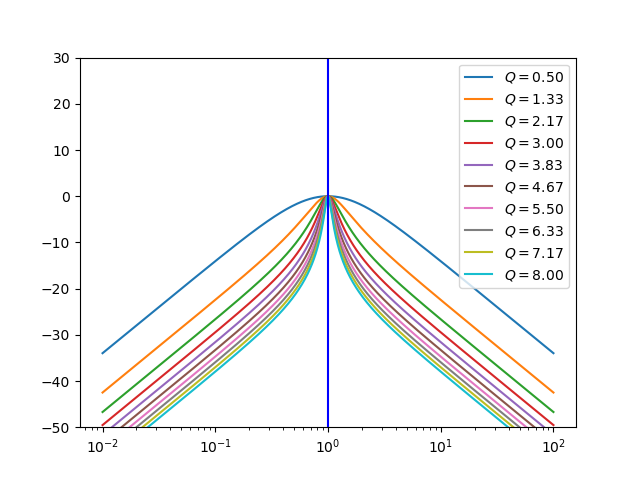
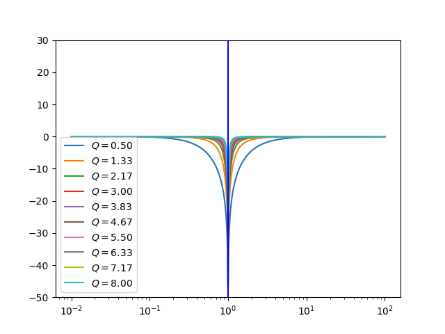
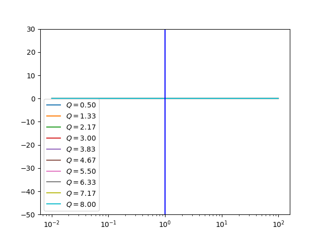
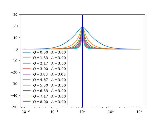
5.4.1.3.2. Second Order Filters from the (Audio) Cookbook

The analog protoypes for filters often used in audio processing are given in the table below. All filters assume a natural frequency \(\w_0=1\).

Show code for figure

import numpy as np
import matplotlib.pyplot as plt
import scipy.signal as sig

plt.close('all')

def H_LP(Q):
    return [[1], [1, 1 / Q, 1]]

def H_HP(Q):
    return [[1, 0, 0], [1, 1/Q, 1]]

def H_BPQ(Q):
    return [[1, 0], [1, 1/Q, 1]]

def H_BP0(Q):
    return [[1/Q, 0], [1, 1/Q, 1]]

def H_Notch(Q):
    return [[1, 0, 1], [1, 1/Q, 1]]

def H_APF(Q):
    return [[1, -1/Q, 1], [1, 1/Q, 1]]

def H_Peak(Q, A):
    return [[1, A/Q, 1], [1, 1/A/Q, 1]]

def H_LS(Q, A):
    return [[A, A * np.sqrt(A) / Q, A**2], [A, np.sqrt(A)/Q, 1]]

def H_HS(Q, A):
    return [[A**2, A * np.sqrt(A) / Q, A], [1, np.sqrt(A)/Q, A]]

filtersQ = [['LP', H_LP, "LPfreqresp"],
           ['HP', H_HP, "HPfreqresp"],
           ['BPQ', H_BPQ, "BPQfreqresp"],
           ['BP0', H_BP0, "BP0freqresp"],
           ['Notch', H_Notch, "Notchfreqresp"],
           ['APF', H_APF, "APFfreqresp"]
           ]
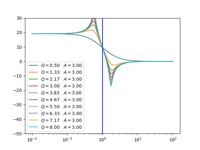
filtersAQ = [['Peak', H_Peak, "peakEQfreqresp"],
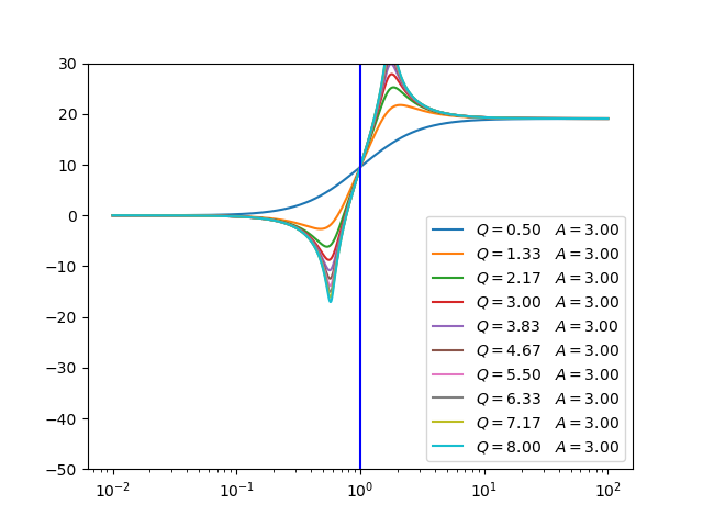
          ['LowShelf', H_LS, 'LowShelffreqresp'],
          ['HighShelf', H_HS, 'HighShelffreqresp']]


Qs = np.linspace(0.5, 8, 10)
for abbr, Hf, name in filtersQ:
    plt.close('all')
    for Q in Qs:
        H = sig.lti(*Hf(Q))
        w, magH = H.freqresp(np.logspace(-2,2,1000))
        plt.plot(w, 20 * np.log10(np.abs(magH)), label=f'$Q = {Q:5.2f}$')

    plt.xscale('log')
    plt.axvline(1, c='blue')
    plt.ylim([-50,30])

    plt.legend()

    plt.savefig("source/figures/" + name + ".png")

for abbr, Hf, name in filtersAQ:
    plt.close('all')
    A = 3
    for Q in Qs:
        H = sig.lti(*Hf(Q, A))
        w, magH = H.freqresp(np.logspace(-2,2,1000))
        plt.plot(w, 20 * np.log10(np.abs(magH)), label=f'$Q = {Q:5.2f}\quad A = {A:5.2f}$')

    plt.xscale('log')
    plt.axvline(1, c='blue')
    plt.ylim([-50,30])

    plt.legend()

    plt.savefig("source/figures/" + name + ".png")

Table 5.2 Analog Second Order Filter Prototypes

Name	Transfer Function	Frequency Response
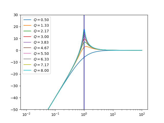
Low pass	\(H(s) = \frac{1}{s^2 + \frac{s}{Q} + 1}\)
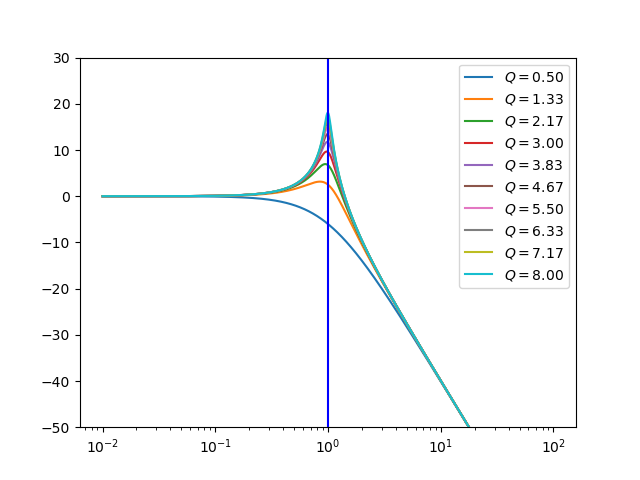
High Pass	\(H(s) = \frac{s^2}{s^2 + \frac{s}{Q} + 1}\)
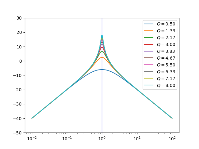
Band Pass (peak gain Q)	\(H(s) = \frac{s}{s^2 + \frac{s}{Q} + 1}\)
Band Pass (peak gain 0dB)	\(H(s) = \frac{\frac{s}{Q}}{s^2 + \frac{s}{Q} + 1}\)
Notch	\(H(s) = \frac{s^2+1}{s^2 + \frac{s}{Q} + 1}\)
APF	\(H(s) = \frac{s^2 - \frac{s}{Q} + 1}{s^2 + \frac{s}{Q} + 1}\)
Peaking EQ	\(H(s) = \frac{s^2 + s\frac{A}{Q} + 1}{s^2 + \frac{s}{AQ} + 1}\)
Low Shelf	\(H(s) = A\frac{s^2 + \frac{\sqrt{A}}{Q}s + A}{As^2 + \frac{\sqrt{A}}{Q}s + 1}\)
High Shelf	\(H(s) = A\frac{As^2 + \frac{\sqrt{A}}{Q}s + 1}{s^2 + \frac{\sqrt{A}}{Q}s + A}\)

5.4.1.4. Higher Order Filters

In some situations higher order filters are needed. The number of free parameters to choose then becomes larger and more diverse filters can be build. Here we look at only one famous example of an \(N\)-th order low pass filter: the Butterworth filter.

The Buttorworth filter is designed in the frequency domain with the following frequency response:

\[|H_n(\w)| = \frac{1}{\sqrt{1+\w^{2n}}}\]

We assume that this frequency response is associated with a filter with a rational transfer function with real coefficients \(H_n(s)\) in the s-domain. This assumption guarantees that the filter can be implemented in analog hardware but also that the filter can be discretized using standard tools (like the bilinear transform to be discussed in a later section). This assumption leads to

\[|H_n(\w)|^2 = H_n(\w) (H_n(\w))^* = H_n(\w) H_n(-\w) = \frac{1}{1+\w^{2n}}\]

Translating this to the s-domain (keep in mind that the frequency response dictates that \(s=j\w\) we get

\[H_n(s) H_n(-s) = \frac{1}{1+(\frac{s}{j})^{2n}} = \frac{1}{1+(-1)^n s^{2n}}\]

The function \(H_n(s) H_n(-s)\) has as poles the solutions of

\[(-1)^n s^{2n} = -1\]

or

\[s^{2n} = (-1)^{n+1} = e^{j\pi(n+1)}\]

and thus writing \(s=r e^{j\phi}\) leads to \(r=1\) and

\[2 n \phi = \pi(n+1) + k 2 \pi\]

i.e.

\[\phi_k = \frac{n+1+2k}{2n}\pi\]

for \(k=0, 1, 2, \ldots, 2n-1\). Leading to the poles

\[p_k = e^{j\phi_k}\]

We plot these roots for \(n=1,2,\ldots,6\)

Show code for figure

import numpy as np
import matplotlib.pyplot as plt
import scipy.signal as sig

plt.close('all')

fig, axs = plt.subplots(1, 6, figsize=(12,2))
for n in np.arange(1, 7):
    circle1 = plt.Circle((0, 0), 1, color='grey', fill=False)
    poles = np.array([np.exp(1j * (n+1+2*k)/(2*n) * np.pi) for k in range(2*n)])
    axs[n-1].add_patch(circle1)
    axs[n-1].scatter(poles.real, poles.imag)
    for k in range(2*n):
        axs[n-1].text(poles[k].real, poles[k].imag, f"{k}")
    axs[n-1].axis('equal')
    axs[n-1].set_title(f"n={n}")

plt.savefig('source/figures/poles_butterworth.png')

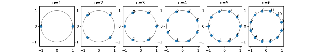
Fig. 5.41 Poles of Butterworth \(H_n(s) H_n(s^*)\). The value of \(k\) is plotted next to all poles.

From the position of the poles (note that if \(s\) is a pole then also \(-s\) is a pole) we see that in case the take \(H_n(s)\) as the system that is characterized only with the poles of \(H(s)H(-s)\) that are in the left half (stable) of the complex plane we end up with a stable filter. Also note that the ‘stable poles’ as those with index \(k=0,\ldots,n-1\). The filter transfer function in the s-domain then becomes:

\[H_n(s) = K \frac{1}{\prod_{k=0}^{n-1} (s - p_k)}\]

It is not too difficult to show that we can set \(K=1\) leading to a filter that has unity gain for \(\w=0\).

The denominator of \(H_n(s)\) is as an \(n\)-th order polynomial in \(s\). On Wikipedia you can find the coefficients of this polynomial in several forms.

Note that the \(s\) transforms to set the corner frequency and the transform to make a lowpass into a highpass filter (end others) are also usable for the Butterworth filter.

Show code for figure

from scipy import signal
import matplotlib.pyplot as plt

plt.close('all')

for order in [2,3,4,5,6,7,8]:
    b, a = signal.butter(order, 100, 'low', analog=True)
    w, h = signal.freqs(b, a)
    plt.semilogx(w, 20 * np.log10(abs(h)), label=f"order {order}")

plt.legend()
plt.title('Butterworth filter frequency response')
plt.xlabel('Frequency [radians / second]')
plt.ylabel('Amplitude [dB]')
plt.margins(0, 0.1)
plt.grid(which='both', axis='both')
plt.axvline(100, color='green') # cutoff frequency

plt.savefig('source/figures/bw_freqresp.png')

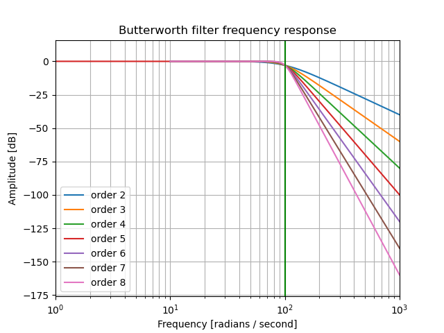
Fig. 5.42 Frequency Response for \(n\)-the order Butterworth Filter.