4.2.1. The \(\ZT\)-Transform¶

4.2.1.1. Definition¶

The Z-transform of a sequence \(x[n]\) is given by

\[X(z) = \sum_{n=-\infty}^{\infty} x[n] z^{-n}\]

For the Z-transform to be meaningful the infinite summation has to converge to a finite value. Convergence of the summation over infinitely many terms is not guaranteed for all values of \(z\). The region of convergence (ROC) defines all values \(z\) for which the Z-transform converges (we say the Z-transform exists for those values of \(z\)). Determining the ROC is not a simple task. In these lecture notes we will most often only state the ROC without proof or use simple rules for systems/signals for which the ROC is known.

The Z-transform is such an important transform in practice because:

Discrete convolution in the time domain corresponds with multiplication in the \(z\)-domain. The Z-transform shares this property with the Fourier transform.
Any difference equation relating input and output of an LTI system is turned into an algebraic equation in \(z\) and the Z-transform of both input and output signal.

Especcially the last property is important in digital signal processing. Difference equations are the important characterizations of digital linear filters in practice.

The above definition of the Z-transform is the bilateral (or two-sided) Z-transform. It takes the sum from \(n=-\infty\) to \(n=+\infty\). The unilateral (or one-sided) Z-transform integrates from \(0\) to \(+\infty\). In signal processing this is a common definition for the Z-transform. In signal processing we are most often interested in causal systems and signals and for such systems both definitions of the Z-transform coincicde.

The inverse Z-transform is a mathematically complex transform. It is given as a line integral:

\[x[n] = \frac{1}{2\pi j}\oint_C X(z)z^{n-1}dz\]

where \(C\) is a closed path containing the origin and entirely in the ROC. Don’t be too much bothered in case you find it hard to see what is going on here. In (digital) signal processing we mostly use Z-transform pairs \(x[n]\ZTright X(z)\) of simple functions without too much use of the definition of the inverse transform.

Table 4.4 **Z-Transform**¶
Synthesis Equation	Analysis Equation
\(x[n] = \frac{1}{2\pi j}\oint_C X(z)z^{n-1}dz\)	\(X(z) = \sum_{n=\infty}^{\infty} x[n] z^{-n}\)

The proof of the synthesis equation given the analysis equation is remarkably simple and follows along the same line of thought as was used in the similar proof for the Fourier transform. This proof is not part of the obligatory theory for this course. The analysis equation is:

\[X(z) = \sum_{k=-\infty}^{\infty} x[k] z^{-k}\]

Multiplying both sides with \(z^{n-1}\) we get:

\[\begin{split}X(z) z^{n-1} &= \left( \sum_{k=-\infty}^{\infty} x[k] z^{-k} \right) z^{n-1}\\ &= \sum_{k=-\infty}^{\infty} x[k] z^{-k+n-1}\end{split}\]

Then integrating along a closed contour that is entirely in the region of convergence of \(X(z)\) and multiplying with \(1/(2\pi j)\) we get:

\[\begin{split}\frac{1}{2\pi j} \oint_C X(z) z^{n-1} dz &= \frac{1}{2\pi j} \oint_C \left(\sum_{k=-\infty}^{\infty} x[k] z^{-k+n-1}\right)dz\\ &= \frac{1}{2\pi j} \sum_{k=-\infty}^{\infty} x[k] \left(\oint_C z^{-(k-n+1)}dz \right)\end{split}\]

Consider the integral in the above expression:

\[\oint_C z^{-m}dz\]

The path C should be entirely in the ROC of \(X(z)\). As a path we select

\[z = r e^{j\phi}\]

the circle around the origin with radius \(r\). The radius \(r\) should be chosen such that the path is within the ROC. The path integral then becomes:

\[\begin{split}\oint_C z^{-m}dz &= \int_{0}^{2\pi} (r e^{j\phi})^{-m} \frac{dz}{d\phi} d\phi\\ &= \int_{0}^{2\pi} r^{-m} e^{-j\phi m} j r e^{j\phi}d\phi\\ &= j r^{1-m} \int_{0}^{2\pi} e^{j\phi (1-m)} d\phi\end{split}\]

For \(m=1\) we get \(2\pi j\) and for \(m\not=1\) the integration is always over one or more periods of the complex exponential and thus the integral is zero. Note that the value of \(r\) is irrelevant as long as it is small enough for the path to be in the ROC.

This leads

\[\begin{split}\frac{1}{2\pi j} \oint_C X(z) z^{n-1} dz &= \frac{1}{2\pi j} \sum_{k=-\infty}^{\infty} x[k] 2\pi j\delta[k-n]\\ &= \sum_{k=-\infty}^{\infty} x[k] \delta[k-n]\\ &= x[n]\end{split}\]

So we have derived the synthesis equation starting from the analysis equation.

4.2.1.2. Eigenfunctions of an LTI System¶

The function \(x[n] = z^{n}\) is an eigenfunction of a LTI system. This follows easily when considering a system with impulse response \(h[n]\) where:

\[h[n] \ZTright H(z)\]

when we feed this system with input \(x[n]=z^n\) the output \(y[n]\) is given by

\[\begin{split}y[n] &= x[n]\ast h[n]\\ &= \sum_{m=-\infty}^{+\infty} h[m] x[n-m]\\ &= \sum_{m=-\infty}^{+\infty} h[m] z^{n-m}\\ &= z^n \sum_{m=-\infty}^{+\infty} h[m] z^{-m}\\ &= H(z) z^n\end{split}\]

So input \(z^n\) leads to output \(H(z)z^n\).

In the eigenfunction \(z^n\) the complex number \(z\) can be written in polair notation as \(z=r e^{j\Omega}\) so that the eigenfunctions are of the form:

\[\begin{split}z^n &= \left( r e^{j\W n} \right)^n\\ &= r^n e^{j\W n}\\ &= r^n \left( \cos(\W n) + j\sin(\W n) \right)\end{split}\]

For \(r<1\) the eigenfunctions are complex combinations of dampened cosine and sine functions.

Show code

import numpy as np
import matplotlib.pyplot as plt

n = np.arange(20)
t = np.arange(0, 20, 0.01)
r = 0.9
x = r**n * np.exp(1j*3*2*np.pi/20*n)
xt = r**t * np.exp(1j*3*2*np.pi/20*t)
fig, axs = plt.subplots(2, sharex=True)
axs[0].stem(n, x.real)
axs[0].plot(t, xt.real, '--')
axs[0].set_ylabel(f"$\Re(z^n)$")

axs[1].stem(n, x.imag)
axs[1].plot(t, xt.imag, '--')
axs[1].set_ylabel(f"$\Im(z^n)$")

plt.savefig('source/figures/dampenedefs.png')

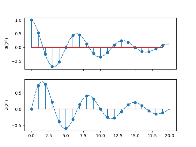
Fig. 4.3 Real and Imaginary Part of Dampened Complex Exponential Function.¶

Observe that for \(r=1\), i.e. \(z=e^{j\W n}\) we get the undampened complex exponentials. The same eigenfunctions we have allready seen when we introduced the Fourier transform. The relation between the \(\ZT\)-transform and the Fourier transform will be further looked at in a subsequent section.

4.2.1.3. Finite and Infinite Signals¶

Consider a finite signal (different from zero in a finite number of samples):

\[x[n] = \begin{matrix}2& \underline{3}& 5& 3& 1 \end{matrix}\]

where we use the convention that the origin (\(n=0\)) is denoted with the underlining and signal values that are not given are equal to zero. The Z-transform equals:

\[X(z) = 2 z^1 + 3 + 5 z^{-1} + 3 z^{-2} + z^{-3}\]

with ROC the entire complex plane without the origin. Now consider an infinite signal

\[x[n] = \begin{matrix}\underline{1}& 0.8& 0.8^2& 0.8^3& 0.8^4& \cdots\end{matrix}\]

with Z-transform:

\[X(z) = \sum_{n=0}^{\infty} 0.8^n z^{-n} = \sum_{n=0}^{\infty} \left(0.8 z^{-1}\right)^n\]

Remember your geometric sequences (meetkundige reeks) from math class? Without proof we state:

\[X(z) = \frac{1}{1-0.8 z^{-1}},\quad |z|>0.8\]

the ROC is \(|z|>0.8\). The ROC follows from the observation that the geometric sequence only converges in case \(|0.8 z^{-1}|<1\). Note that not all infinite signals result in a finite Z-transform (in fact, most infinite signals do not have bounded Z-transform).

The second example can be summarized as:

\[0.8^n u[n] \ZTright \frac{1}{1-0.8 z^{-1}},\quad |z|>0.8.\]

4.2.1.4. The Z-Transform and the Fourier Transform¶

Remember the discrete time Fourier transform (DTFT):

\[X(\W) = \sum_{n=-\infty}^{\infty} x[n] e^{-j\W n}\]

Comparing the above with the definition of the Z-transform \(X(z)\) we see that

\[X(z)\Bigr|_{z=e^{j\W}} = X(\W)\]

i.e. the Fourier transform can be found from the Z-transform along the unit circle in the complex domain.

Given that we have already established that the DTFT contains as much information as the original signal (obvious since there exists an inverse DTFT) the question arises what the use for the Z-transform is. There are more than one reason why the Z-transform is a handy tool in the analysis of systems and signals:

Where the Fourier transform is very capable of describing signals that are periodical in nature, it has difficulties in describing signals that show a transient behavior. The Z-transform is more suited for such signals.
Perhaps the most important reason for the value of the Z-transform is its link with linear systems described by a difference equation (see this section). In a subsequent section we will show that using the Z-transform a difference equation in the time domain can be written as an algebraic equation that is more easily dealt with.