2.4. Eigenfunctions
A remarkable fact of linear systems is that the complex exponentials are eigenfunctions of a linear system. I.e. if we take a complex exponential \(x(t)=\exp(j\omega t)\) as input, the output is a complex exponential, with the same frequency as the input but multiplied with a complex constant (dependent on the frequency).
Fig. 2.12 Complex Exponentials are the Eigenfunctions of a CT LTI Linear System
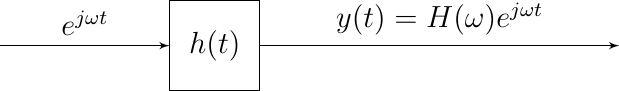
Consider the system with impulse response \(h\) then the output is given by:
We can simplify this as
Observe that the integral only depends on \(\omega\) and we denote it as \(H(\omega)\), then:
i.e. in case the input of a linear system is a sinusoidal signal (complex exponential) the output is the exponential function (sinusoidal function with the same frequency) multiplied with a complex factor \(H(\omega)\) that is completely characterized by the linear system (its impulse response).
The function \(H\)
is called the Fourier transform of \(h\). The Fourier transform will play a major role in this lecture series.
Let’s redo this analysis for a real valued function: \(x(t)=\cos(\w t)\). We know that
Because we are considering a linear system we have:
Note that from the definition of the Fourier transform (Eq. (2.2))we can see that if \(h\) is real valued function (which in practice it always is) that \(H(-\w) = H^\star(\w)\). Writing \(H(\w)\) in polar notation:
So
So for a linear system with impulse response \(h\) we have
and
Evidently the use of complex exponential functions allows for a much more convenient (and short) notation. Complex numbers are really indispensible in signal processing theory.