FIR Filters

A finite impulse response filter is a filter whose impulse response function \(h[n]\) is non zero on a bounded subset of \(\setR\), i.e. \(h[n]=0\) for \(|n|>N\).

The digital filter then is implemented as a convolution:

\[\begin{split}y[n] &= x[n] \ast h[n]\\ &= \sum_{k=-\infty}^{\infty} x[n-k] h[k]\end{split}\]

In the Z-domain a FIR filter is characterized as:

\[H(z) = \sum_{n=-\infty}^{\infty} h[n] z^{-n}\]

Designing a FIR filter then boils down to the choice of the impulse response function \(h[n]\).

Simple Filter

Consider the following causal FIR filter:

\[y[n] = x[n-2] + 2 x[n-1] + x[n]\]

The impulse response is:

\[h[n] = (\underline{1}\;2\;1)\]

The DTFT is then given as:

\[\begin{split}H(\W) &= 1 + 2 e^{-j\W} + e^{-2j\W}\\ &= e^{-j\W}\left( e^{j\W} + 2 + e^{-j\W}\right)\\ &= e^{-j\W}\left(2+2\cos(\W)\right)\end{split}\]

We thus see that:

\[\begin{split}|H(\W)| &= 2+2\cos(\W)\\ \angle\W &= -\W\end{split}\]

Now consider a cosine inout signal:

\[x[n] = \cos(\W_0 n)\]

The output then is

\[y[n] = |H(\W_0)| \cos\left(\W_0 n + \angle H(\W_0)\right)\]

Below we check this in Python:

Show code for figure

import numpy as np
import matplotlib.pyplot as plt

n = np.arange(32)
t = np.linspace(0,32,1000)
hn = np.array([0,0,1,2,1]) # to make the first 1 the origin when convolving
W0 = np.pi/6
xn = np.cos(W0 * n)
xt = np.cos(W0 * t)

fig, axs = plt.subplots(2)
axs[0].plot(t, xt, '--');
axs[0].stem(n, xn, use_line_collection=True);

H = lambda W: np.exp(-1j*W) * (2 + 2*np.cos(W))

absW0 = np.abs(H(W0))
print("Gain: %5.2f" % absW0)
angleW0 = np.angle(H(W0))
print("Angle: %5.2f" % angleW0)
yt_theory = absW0 * np.cos(W0*t + angleW0)
yn = np.convolve(xn, hn, mode='same')
axs[1].plot(t, yt_theory, '--');
axs[1].stem(n, yn, use_line_collection=True);

plt.savefig('source/figures/discretetimeconvolution121.png')

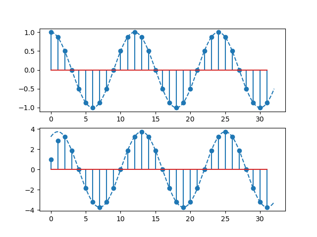
FIR convolution filtering of cosine with kernel \(h=\{\underline{1}\;1\;1\}\)

Convince yourself using the figure above that theory indeed predicts practice. Except for the first two samples of \(y[n]\), why is that?

Running Average Filter

Another simple FIR filter is to calculate the average of \(K\) consecutive samples, for \(K=5\) we get:

\[\begin{split}y[n] &= \frac{1}{5}\left( x[n-2] + x[n-1] + x[n] + x[n+1] + x[n+2]\right)\\ &= x[n] \ast h[n]\end{split}\]

where

\[h[n] = (1\;1\;\underline{1}\;1\;1)\]

The discrete time Fourier transform is:

\[\begin{split}H(\W) &= \sum_{n=-\infty}^{\infty} h[n] e^{-j \W n}\\ &= \frac{1}{5} \left( e^{j 2 \W} + e^{j \W} + 1 + e^{-j\W} + e^{-j2\W} \right)\\ &= \frac{1}{5} \left( 1 + 2\cos(\W) + 2\cos(2\W) \right)\end{split}\]

On the interval \(\W\in[-\pi,\pi]\) the frequency response looks like:

Show code for figure

plt.close('all')
W = np.linspace(-np.pi, np.pi, 1000)
H = 1/5*(1 + 2*np.cos(W) + 2*np.cos(2*W))
plt.plot(W,H)

plt.savefig('source/figures/freqresp5pointaverage.png')

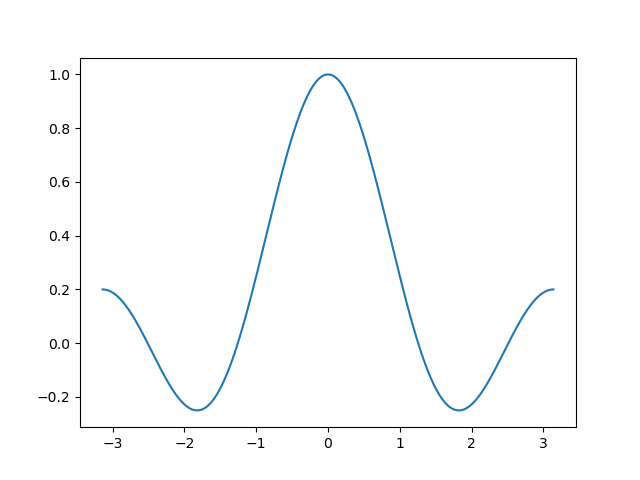
Frequency response of 5 point average filter

From the plot it is evident that there are 4 zeros in the frequency response. Of course we could set \(H\W)=0\) and calculate those zeros. However we do so by analyzing this filter in the Z-domain.

\[\begin{split}H(z) &= \sum_{n=-\infty}^{\infty} x[n] z^{-n}\\ &= \frac{1}{5}\left( z^2 + z + 1 + z^{-1} + z^{-2}\right)\\ &= \frac{ \frac{1}{5} \left( 1 + z + z^2 + z^3 + z^4\right)}{z^2}\end{split}\]

Using the sum formula for a geometric sequence we get

\[\begin{split}H(z) &= \frac{\frac{1}{5} \frac{1-z^5}{1-z}}{z^2}\\ &= \frac{1}{5} \frac{1-z^5}{z^2(1-z)}\end{split}\]

Note that the zero in \(z=1\) cancels the pole in \(z=1\) so we are left with four zeros (obtained as solutions of \(z^5=1\) excluding the solution \(z=1\)). The four zeros are at \(z=\pm\pi/5\) and \(z=\pm 2\pi/5\).

A 5 tap running average filter. Poles and Zeros plot and Frequency Resppnse plot.

Design in the Frequency Domain

In this section we discuss the design based on frequency domain considerations. Suppose we want to approximate an ideal band-pass filter with unit gain for frequencies between \(\Omega_\text{low}\) and \(\Omega_\text{high}\).

Note that due to the symmetry \(H(-\Omega)=H(\Omega)\) the mathemetical formulation is:

\[H(\Omega) = u(\Omega+\Omega_\text{high}) - u(\Omega+\Omega_\text{low}) + u(\Omega-\Omega_\text{low}) - u(\Omega-\Omega_\text{high})\]

The inverse Fourier transform then gives:

\[\begin{split}h[n] &= \frac{1}{2\pi} \int_{\langle 2\pi \rangle} X(\Omega)e^{j\Omega n}d\Omega\\ &= \frac{1}{2\pi} \left( \int_{\Omega_\text{low}}^{\Omega_\text{high}} e^{j\Omega n} d\Omega + \int_{-\Omega_\text{high}}^{-\Omega_\text{low}} e^{j\Omega n} d\Omega \right)\\ &= \frac{1}{2\pi} \left( \frac{1}{jt} \left[e^{j\Omega n}\right]_{\Omega_\text{low}}^{\Omega_\text{high}} + \frac{1}{jn} \left[e^{j\Omega n}\right]_{-\Omega_\text{high}}^{-\Omega_\text{low}} \right)\\ &= \frac{1}{2\pi} \frac{1}{jn} \left( e^{j\Omega_\text{high}n} - e^{j\Omega_\text{low}n} + e^{-j\Omega_\text{low}n} - e^{-j\Omega_\text{high}n} \right)\\ &= \frac{1}{\pi n}\left( \frac{e^{j\Omega_\text{high}n} - e^{j\Omega_\text{high}n}}{2j} - \frac{e^{j\Omega_\text{low}n} - e^{-j\Omega_\text{low}n}}{2j}\right)\\ &= \frac{\sin(\Omega_\text{high}n)}{\pi n} - \frac{\sin(\Omega_\text{low}n)}{\pi n}\\ &= \frac{\Omega_\text{high}}{\pi}\sinc\left(\frac{\Omega_\text{high}}{\pi} n\right) - \frac{\Omega_\text{low}}{\pi}\sinc\left(\frac{\Omega_\text{low}}{\pi} n\right)\end{split}\]

Note that the sinc function is defined as \(\sinc(t) = \sin(\pi t)/(\pi t)\), this is also the definition used in Numpy.

In the code and plot below the formula above is used to generate \(h[n]\) for a bandpass filter. The goal is to design a bandpass filter working on discrete signals for which the sampling frequency is 44100 Hz. The band start at low frequency 100 Hz and end at high frequency 4000 Hz. Be sure you understand how to get from frequency \(f\) in Hz to radial frequency \(\Omega\). Refer to the section on the DTFT.

Show code for figure

plt.close('all')

fs = 44100
flow = 100
fhigh = 4000

N = 32
n = np.arange(-N, N+1)
Omega_low = 2*np.pi*flow/fs
Omega_high = 2*np.pi*fhigh/fs
h = Omega_high/np.pi * np.sinc(Omega_high/np.pi * n) - \
          Omega_low/np.pi * np.sinc(Omega_low/np.pi * n)

plt.stem(n, h, use_line_collection=True);

# to check our code we compare it with firwin (with the right set of parameters)
numtaps = 2*N+1
from scipy.signal import firwin
hfirwin = firwin(numtaps, [flow, fhigh], pass_zero=False, fs=fs, window='boxcar', scale=False)
print("Calculated h[n] equal to result from 'firwin' ?  ", np.allclose(h, hfirwin))

plt.savefig('source/figures/discrete_bandpass_impulse_response.png')

Calculated h[n] equal to result from 'firwin' ?   True

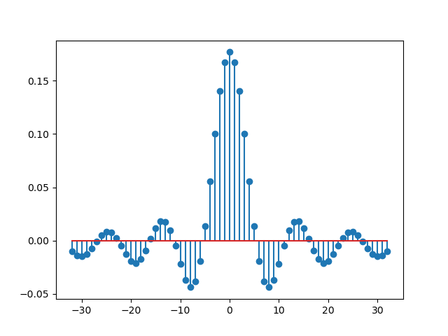
Bandpass Filter Impulse Response.

In the code above there is a correctness check. The impulse response is compared with the impulse response calculated by the function scipy.signal.firwin.

It should also be noted that the number of taps (65 in the example above) is too small: the sinc functions are still fluctuating with relative large amplitude for \(|n|=32\). The frequency response therefore will not be that for an ideal bandpass filter.

Show code for figure

plt.close('all')

from FIRfilters import test_bandpass
test_bandpass()

plt.savefig('source/figures/bandpass_sweep.png')

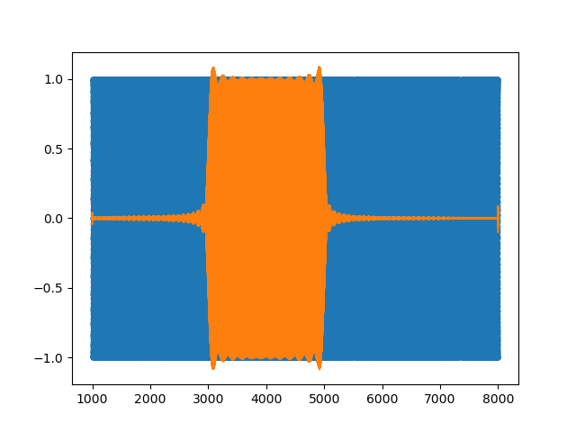
Bandpass Filter Response on a Chirp Signal.

In blue the chirp signal is shown. The time sampling is 44100 Hz and the total duration of the signal is 3s, therefore the entire plot is blue for the interval from -1 to 1. The instantaneous frequency in the signal ranges linearly from 1000 to 3000 Hz. Instead of the time the corresponding frequency is shown on the x-axis.

In orange the response \(x[n]\ast h[n]\) is shown. From the figure it is evident that the filter works as a bandpass filter. Also note that it is not an ideal bandpass filter as we had to truncate the impulse response.

The code for this ezample is given below

"""Finite Impulse Filters."""
import numpy as np
import matplotlib.pyplot as plt


def FIRlow(W, N):
    """Low pass filter kernel."""
    n = np.arange(-N, N + 1)
    return W / np.pi * np.sinc(W / np.pi * n)


def test(n):
    """Simple test."""
    x = np.arange(10)
    print(x)


def FIRbandpass(Wlow, Whigh, N):
    """Return convolution kernel for bandpass filter."""
    return FIRlow(Whigh, N) - FIRlow(Wlow, N)


def f2W(f, fs):
    """From freq in hz to freq in rad/s."""
    return 2 * np.pi * f / fs


def generate_chirp(startf, endf, fs, duration):
    """Generate chirp signal."""
    N = int(duration * fs)
    t = np.linspace(0, duration, N)
    phase = 2 * np.pi * (startf * t + (endf - startf) / duration / 2 * t**2)
    ft = startf + (endf-startf) / duration*t
    return t, ft, np.sin(phase)


def test_bandpass():
    """Test the bandpass filter by feeding it a chirp signal."""
    t, ft, x = generate_chirp(1000.0, 8000.0, 44100.0, 3.0)
    plt.plot(ft, x, '.-')

    fs = 44100
    flow = 3000
    fhigh = 5000
    N = 256
    w = FIRbandpass(f2W(flow, fs), f2W(fhigh, fs), N)
    y = np.convolve(x, w, mode='same')
    plt.plot(ft, y)


if __name__=='__main__':
    test_bandpass()
    plt.show()