IIR Filters
Infinite impulse response filters are characterized with a difference equation like:
as discussed in the second chapter on LTI systems. There we have shown that for instance a simple system characterized with
corresponds with an LTI system with an infinite impulse response:
and we have established that it is a stable filter in case \(|\alpha|<1\). In this section we will analyze these IIR filters in the Z-domain.
Setting \(a_0=1\) the difference equation at the top can be rewritten as:
Applying the Z-transform to both sides (and using the shift property) we get
or
In these notes we are going to restrict ourselves to the case \(M\leq 2\) and \(N\leq2\). In audio processing such a digital filter is called a biquad filter.
The first expression if the starting point to represent the filter as a block diagram. The second form is starting point for poles-zeros analysis of the filter.
The analysis in the Z-domain is done through some examples of digital filters. Consider the filter defined with difference equation
Leading to the transfer function \(H(z)\):
The pole of this filter is at \(z=\alpha\) and thus the filter is stable for \(\alpha<1\).
The frequency response of the filter can be found by substituting \(e^{j\W}\) for \(z\) in the transfer function:
Show code for figure
1import numpy as np
2import matplotlib.pyplot as plt
3from audiolazy import z
4
5Hlow = 1/(1-0.8*z**(-1))
6Hlow.plot(freq_scale='log', rate=44100)
7plt.savefig('source/figures/lowpassresppnse.png')
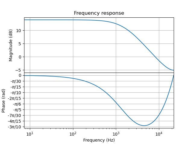
Lowpass Response of Filter with transfer function \(H(z) = \frac{1}{1-0.8 z^{-1}}\)