Bodeplots in Python
DIY Python
Consider the (angular) frequency reponse function of a low-pass filter:
where \(\omega_c\) is the cut-off frequency. In a Bode magnitude plot we plot the magnitude (in decibels) of the transfer function (frequency response), i.e.
Be sure you can do these steps yourself, especcially the last step is not trivial!
Most often in plots we plot ‘real’ frequencies and not angular frequencies. Remember that \(\omega = 2\pi f\). The cut-off frequency is taken at 2KHz leading to \(\omega_c = 4000\pi\). We may write a simple python function to represent the transfer function:
In [1]: from pylab import *

In [2]: def H(w):
   ...:     wc = 4000*pi
   ...:     return 1.0 / (1.0 + 1j * w / wc)
   ...:
and then plot it:
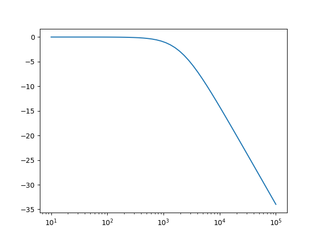
In [3]: f = logspace(1,5) # frequencies from 10**1 to 10**5

In [4]: plot(f, 20*log10(abs(H(2*pi*f)))); xscale('log')

Observe that the corner (or cut-off) frequency is at around 2000 kHz and that the decay above that frequency is 20 dB per decade (equal to 6 dB per octave).
Scipy Signal Processing Package
Scipy also contains functions to represent continuous time linear systems. An LTI system is specified in the \(s\)-domain. For the low-pass filter we have used in the previous section the transfer function is:
In [5]: from pylab import *

In [6]: from scipy import signal

In [7]: system = signal.lti([1], [1/(4000*pi),1])

In [8]: f = logspace(1, 5)

In [9]: w = 2 * pi * f

In [10]: w, mag, phase = signal.bode(system,w)

In [11]: semilogx( f, mag);